Interactions and ANOVA
Note: This script is based heavily on Jonathan Taylor’s class notes https://web.stanford.edu/class/stats191/notebooks/Interactions.html
Download and format data:
[1]:
%matplotlib inline
[2]:
import os
import shutil

import numpy as np
import requests

np.set_printoptions(precision=4, suppress=True)

import pandas as pd

pd.set_option("display.width", 100)
import matplotlib.pyplot as plt
from statsmodels.formula.api import ols
from statsmodels.graphics.api import abline_plot, interaction_plot
from statsmodels.stats.anova import anova_lm


def download_file(url, mode="t"):
    local_filename = url.split("/")[-1]
    if os.path.exists(local_filename):
        return local_filename
    with requests.get(url, stream=True) as r:
        with open(local_filename, f"w{mode}") as f:
            f.write(r.text)
    return local_filename


url = "https://raw.githubusercontent.com/statsmodels/smdatasets/main/data/anova/salary/salary.table"
salary_table = pd.read_csv(download_file(url), sep="\t")

E = salary_table.E
M = salary_table.M
X = salary_table.X
S = salary_table.S
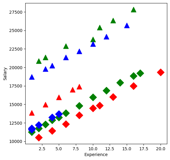
Take a look at the data:
[3]:
plt.figure(figsize=(6, 6))
symbols = ["D", "^"]
colors = ["r", "g", "blue"]
factor_groups = salary_table.groupby(["E", "M"])
for values, group in factor_groups:
    i, j = values
    plt.scatter(group["X"], group["S"], marker=symbols[j], color=colors[i - 1], s=144)
plt.xlabel("Experience")
plt.ylabel("Salary")
[3]:
Text(0, 0.5, 'Salary')
Fit a linear model:
[4]:
formula = "S ~ C(E) + C(M) + X"
lm = ols(formula, salary_table).fit()
print(lm.summary())
                            OLS Regression Results
==============================================================================
Dep. Variable:                      S   R-squared:                       0.957
Model:                            OLS   Adj. R-squared:                  0.953
Method:                 Least Squares   F-statistic:                     226.8
Date:                Fri, 05 Dec 2025   Prob (F-statistic):           2.23e-27
Time:                        18:15:21   Log-Likelihood:                -381.63
No. Observations:                  46   AIC:                             773.3
Df Residuals:                      41   BIC:                             782.4
Df Model:                           4
Covariance Type:            nonrobust
==============================================================================
                 coef    std err          t      P>|t|      [0.025      0.975]
------------------------------------------------------------------------------
Intercept   8035.5976    386.689     20.781      0.000    7254.663    8816.532
C(E)[T.2]   3144.0352    361.968      8.686      0.000    2413.025    3875.045
C(E)[T.3]   2996.2103    411.753      7.277      0.000    2164.659    3827.762
C(M)[T.1]   6883.5310    313.919     21.928      0.000    6249.559    7517.503
X            546.1840     30.519     17.896      0.000     484.549     607.819
==============================================================================
Omnibus:                        2.293   Durbin-Watson:                   2.237
Prob(Omnibus):                  0.318   Jarque-Bera (JB):                1.362
Skew:                          -0.077   Prob(JB):                        0.506
Kurtosis:                       2.171   Cond. No.                         33.5
==============================================================================

Notes:
[1] Standard Errors assume that the covariance matrix of the errors is correctly specified.
Have a look at the created design matrix:
[5]:
lm.model.exog[:5]
[5]:
array([[1., 0., 0., 1., 1.],
       [1., 0., 1., 0., 1.],
       [1., 0., 1., 1., 1.],
       [1., 1., 0., 0., 1.],
       [1., 0., 1., 0., 1.]])
Or since we initially passed in a DataFrame, we have a DataFrame available in
[6]:
lm.model.data.orig_exog[:5]
[6]:
| Intercept | C(E)[T.2] | C(E)[T.3] | C(M)[T.1] | X | |
|---|---|---|---|---|---|
| 0 | 1.0 | 0.0 | 0.0 | 1.0 | 1.0 |
| 1 | 1.0 | 0.0 | 1.0 | 0.0 | 1.0 |
| 2 | 1.0 | 0.0 | 1.0 | 1.0 | 1.0 |
| 3 | 1.0 | 1.0 | 0.0 | 0.0 | 1.0 |
| 4 | 1.0 | 0.0 | 1.0 | 0.0 | 1.0 |
We keep a reference to the original untouched data in
[7]:
lm.model.data.frame[:5]
[7]:
| S | X | E | M | |
|---|---|---|---|---|
| 0 | 13876 | 1 | 1 | 1 |
| 1 | 11608 | 1 | 3 | 0 |
| 2 | 18701 | 1 | 3 | 1 |
| 3 | 11283 | 1 | 2 | 0 |
| 4 | 11767 | 1 | 3 | 0 |
Influence statistics
[8]:
infl = lm.get_influence()
print(infl.summary_table())
==================================================================================================
       obs      endog     fitted     Cook's   student.   hat diag    dffits   ext.stud.     dffits
                           value          d   residual              internal   residual
--------------------------------------------------------------------------------------------------
         0  13876.000  15465.313      0.104     -1.683      0.155     -0.722     -1.723     -0.739
         1  11608.000  11577.992      0.000      0.031      0.130      0.012      0.031      0.012
         2  18701.000  18461.523      0.001      0.247      0.109      0.086      0.244      0.085
         3  11283.000  11725.817      0.005     -0.458      0.113     -0.163     -0.453     -0.162
         4  11767.000  11577.992      0.001      0.197      0.130      0.076      0.195      0.075
         5  20872.000  19155.532      0.092      1.787      0.126      0.678      1.838      0.698
         6  11772.000  12272.001      0.006     -0.513      0.101     -0.172     -0.509     -0.170
         7  10535.000   9127.966      0.056      1.457      0.116      0.529      1.478      0.537
         8  12195.000  12124.176      0.000      0.074      0.123      0.028      0.073      0.027
         9  12313.000  12818.185      0.005     -0.516      0.091     -0.163     -0.511     -0.161
        10  14975.000  16557.681      0.084     -1.655      0.134     -0.650     -1.692     -0.664
        11  21371.000  19701.716      0.078      1.728      0.116      0.624      1.772      0.640
        12  19800.000  19553.891      0.001      0.252      0.096      0.082      0.249      0.081
        13  11417.000  10220.334      0.033      1.227      0.098      0.405      1.234      0.408
        14  20263.000  20100.075      0.001      0.166      0.093      0.053      0.165      0.053
        15  13231.000  13216.544      0.000      0.015      0.114      0.005      0.015      0.005
        16  12884.000  13364.369      0.004     -0.488      0.082     -0.146     -0.483     -0.145
        17  13245.000  13910.553      0.007     -0.674      0.075     -0.192     -0.669     -0.191
        18  13677.000  13762.728      0.000     -0.089      0.113     -0.032     -0.087     -0.031
        19  15965.000  17650.049      0.082     -1.747      0.119     -0.642     -1.794     -0.659
        20  12336.000  11312.702      0.021      1.043      0.087      0.323      1.044      0.323
        21  21352.000  21192.443      0.001      0.163      0.091      0.052      0.161      0.051
        22  13839.000  14456.737      0.006     -0.624      0.070     -0.171     -0.619     -0.170
        23  22884.000  21340.268      0.052      1.579      0.095      0.511      1.610      0.521
        24  16978.000  18742.417      0.083     -1.822      0.111     -0.644     -1.877     -0.664
        25  14803.000  15549.105      0.008     -0.751      0.065     -0.199     -0.747     -0.198
        26  17404.000  19288.601      0.093     -1.944      0.110     -0.684     -2.016     -0.709
        27  22184.000  22284.811      0.000     -0.103      0.096     -0.034     -0.102     -0.033
        28  13548.000  12405.070      0.025      1.162      0.083      0.350      1.167      0.352
        29  14467.000  13497.438      0.018      0.987      0.086      0.304      0.987      0.304
        30  15942.000  16641.473      0.007     -0.705      0.068     -0.190     -0.701     -0.189
        31  23174.000  23377.179      0.001     -0.209      0.108     -0.073     -0.207     -0.072
        32  23780.000  23525.004      0.001      0.260      0.092      0.083      0.257      0.082
        33  25410.000  24071.188      0.040      1.370      0.096      0.446      1.386      0.451
        34  14861.000  14043.622      0.014      0.834      0.091      0.263      0.831      0.262
        35  16882.000  17733.841      0.012     -0.863      0.077     -0.249     -0.860     -0.249
        36  24170.000  24469.547      0.003     -0.312      0.127     -0.119     -0.309     -0.118
        37  15990.000  15135.990      0.018      0.878      0.104      0.300      0.876      0.299
        38  26330.000  25163.556      0.035      1.202      0.109      0.420      1.209      0.422
        39  17949.000  18826.209      0.017     -0.897      0.093     -0.288     -0.895     -0.287
        40  25685.000  26108.099      0.008     -0.452      0.169     -0.204     -0.447     -0.202
        41  27837.000  26802.108      0.039      1.087      0.141      0.440      1.089      0.441
        42  18838.000  19918.577      0.033     -1.119      0.117     -0.407     -1.123     -0.408
        43  17483.000  16774.542      0.018      0.743      0.138      0.297      0.739      0.295
        44  19207.000  20464.761      0.052     -1.313      0.131     -0.511     -1.325     -0.515
        45  19346.000  18959.278      0.009      0.423      0.208      0.216      0.419      0.214
==================================================================================================
or get a dataframe
[9]:
df_infl = infl.summary_frame()
[10]:
df_infl[:5]
[10]:
| dfb_Intercept | dfb_C(E)[T.2] | dfb_C(E)[T.3] | dfb_C(M)[T.1] | dfb_X | cooks_d | standard_resid | hat_diag | dffits_internal | student_resid | dffits | |
|---|---|---|---|---|---|---|---|---|---|---|---|
| 0 | -0.505123 | 0.376134 | 0.483977 | -0.369677 | 0.399111 | 0.104186 | -1.683099 | 0.155327 | -0.721753 | -1.723037 | -0.738880 |
| 1 | 0.004663 | 0.000145 | 0.006733 | -0.006220 | -0.004449 | 0.000029 | 0.031318 | 0.130266 | 0.012120 | 0.030934 | 0.011972 |
| 2 | 0.013627 | 0.000367 | 0.036876 | 0.030514 | -0.034970 | 0.001492 | 0.246931 | 0.109021 | 0.086377 | 0.244082 | 0.085380 |
| 3 | -0.083152 | -0.074411 | 0.009704 | 0.053783 | 0.105122 | 0.005338 | -0.457630 | 0.113030 | -0.163364 | -0.453173 | -0.161773 |
| 4 | 0.029382 | 0.000917 | 0.042425 | -0.039198 | -0.028036 | 0.001166 | 0.197257 | 0.130266 | 0.076340 | 0.194929 | 0.075439 |
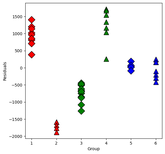
Now plot the residuals within the groups separately:
[11]:
resid = lm.resid
plt.figure(figsize=(6, 6))
for values, group in factor_groups:
    i, j = values
    group_num = i * 2 + j - 1  # for plotting purposes
    x = [group_num] * len(group)
    plt.scatter(
        x,
        resid[group.index],
        marker=symbols[j],
        color=colors[i - 1],
        s=144,
        edgecolors="black",
    )
plt.xlabel("Group")
plt.ylabel("Residuals")
[11]:
Text(0, 0.5, 'Residuals')
Now we will test some interactions using anova or f_test
[12]:
interX_lm = ols("S ~ C(E) * X + C(M)", salary_table).fit()
print(interX_lm.summary())
                            OLS Regression Results
==============================================================================
Dep. Variable:                      S   R-squared:                       0.961
Model:                            OLS   Adj. R-squared:                  0.955
Method:                 Least Squares   F-statistic:                     158.6
Date:                Fri, 05 Dec 2025   Prob (F-statistic):           8.23e-26
Time:                        18:15:21   Log-Likelihood:                -379.47
No. Observations:                  46   AIC:                             772.9
Df Residuals:                      39   BIC:                             785.7
Df Model:                           6
Covariance Type:            nonrobust
===============================================================================
                  coef    std err          t      P>|t|      [0.025      0.975]
-------------------------------------------------------------------------------
Intercept    7256.2800    549.494     13.205      0.000    6144.824    8367.736
C(E)[T.2]    4172.5045    674.966      6.182      0.000    2807.256    5537.753
C(E)[T.3]    3946.3649    686.693      5.747      0.000    2557.396    5335.333
C(M)[T.1]    7102.4539    333.442     21.300      0.000    6428.005    7776.903
X             632.2878     53.185     11.888      0.000     524.710     739.865
C(E)[T.2]:X  -125.5147     69.863     -1.797      0.080    -266.826      15.796
C(E)[T.3]:X  -141.2741     89.281     -1.582      0.122    -321.861      39.313
==============================================================================
Omnibus:                        0.432   Durbin-Watson:                   2.179
Prob(Omnibus):                  0.806   Jarque-Bera (JB):                0.590
Skew:                           0.144   Prob(JB):                        0.744
Kurtosis:                       2.526   Cond. No.                         69.7
==============================================================================

Notes:
[1] Standard Errors assume that the covariance matrix of the errors is correctly specified.
Do an ANOVA check
[13]:
from statsmodels.stats.api import anova_lm

table1 = anova_lm(lm, interX_lm)
print(table1)

interM_lm = ols("S ~ X + C(E)*C(M)", data=salary_table).fit()
print(interM_lm.summary())

table2 = anova_lm(lm, interM_lm)
print(table2)
   df_resid           ssr  df_diff       ss_diff         F    Pr(>F)
0      41.0  4.328072e+07      0.0           NaN       NaN       NaN
1      39.0  3.941068e+07      2.0  3.870040e+06  1.914856  0.160964
                            OLS Regression Results
==============================================================================
Dep. Variable:                      S   R-squared:                       0.999
Model:                            OLS   Adj. R-squared:                  0.999
Method:                 Least Squares   F-statistic:                     5517.
Date:                Fri, 05 Dec 2025   Prob (F-statistic):           1.67e-55
Time:                        18:15:22   Log-Likelihood:                -298.74
No. Observations:                  46   AIC:                             611.5
Df Residuals:                      39   BIC:                             624.3
Df Model:                           6
Covariance Type:            nonrobust
=======================================================================================
                          coef    std err          t      P>|t|      [0.025      0.975]
---------------------------------------------------------------------------------------
Intercept            9472.6854     80.344    117.902      0.000    9310.175    9635.196
C(E)[T.2]            1381.6706     77.319     17.870      0.000    1225.279    1538.063
C(E)[T.3]            1730.7483    105.334     16.431      0.000    1517.690    1943.806
C(M)[T.1]            3981.3769    101.175     39.351      0.000    3776.732    4186.022
C(E)[T.2]:C(M)[T.1]  4902.5231    131.359     37.322      0.000    4636.825    5168.222
C(E)[T.3]:C(M)[T.1]  3066.0351    149.330     20.532      0.000    2763.986    3368.084
X                     496.9870      5.566     89.283      0.000     485.728     508.246
==============================================================================
Omnibus:                       74.761   Durbin-Watson:                   2.244
Prob(Omnibus):                  0.000   Jarque-Bera (JB):             1037.873
Skew:                          -4.103   Prob(JB):                    4.25e-226
Kurtosis:                      24.776   Cond. No.                         79.0
==============================================================================

Notes:
[1] Standard Errors assume that the covariance matrix of the errors is correctly specified.
   df_resid           ssr  df_diff       ss_diff           F        Pr(>F)
0      41.0  4.328072e+07      0.0           NaN         NaN           NaN
1      39.0  1.178168e+06      2.0  4.210255e+07  696.844466  3.025504e-31
The design matrix as a DataFrame
[14]:
interM_lm.model.data.orig_exog[:5]
[14]:
| Intercept | C(E)[T.2] | C(E)[T.3] | C(M)[T.1] | C(E)[T.2]:C(M)[T.1] | C(E)[T.3]:C(M)[T.1] | X | |
|---|---|---|---|---|---|---|---|
| 0 | 1.0 | 0.0 | 0.0 | 1.0 | 0.0 | 0.0 | 1.0 |
| 1 | 1.0 | 0.0 | 1.0 | 0.0 | 0.0 | 0.0 | 1.0 |
| 2 | 1.0 | 0.0 | 1.0 | 1.0 | 0.0 | 1.0 | 1.0 |
| 3 | 1.0 | 1.0 | 0.0 | 0.0 | 0.0 | 0.0 | 1.0 |
| 4 | 1.0 | 0.0 | 1.0 | 0.0 | 0.0 | 0.0 | 1.0 |
The design matrix as an ndarray
[15]:
interM_lm.model.exog
interM_lm.model.exog_names
[15]:
['Intercept',
 'C(E)[T.2]',
 'C(E)[T.3]',
 'C(M)[T.1]',
 'C(E)[T.2]:C(M)[T.1]',
 'C(E)[T.3]:C(M)[T.1]',
 'X']
[16]:
infl = interM_lm.get_influence()
resid = infl.resid_studentized_internal
plt.figure(figsize=(6, 6))
for values, group in factor_groups:
    i, j = values
    idx = group.index
    plt.scatter(
        X[idx],
        resid[idx],
        marker=symbols[j],
        color=colors[i - 1],
        s=144,
        edgecolors="black",
    )
plt.xlabel("X")
plt.ylabel("standardized resids")
[16]:
Text(0, 0.5, 'standardized resids')
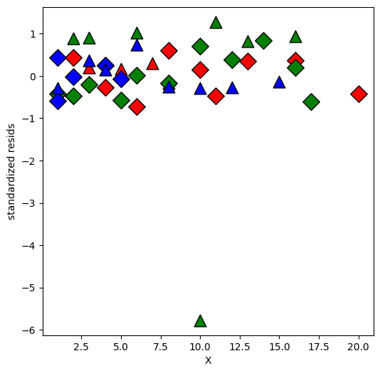
Looks like one observation is an outlier.
[17]:
drop_idx = abs(resid).argmax()
print(drop_idx)  # zero-based index
idx = salary_table.index.drop(drop_idx)

lm32 = ols("S ~ C(E) + X + C(M)", data=salary_table, subset=idx).fit()

print(lm32.summary())
print("\n")

interX_lm32 = ols("S ~ C(E) * X + C(M)", data=salary_table, subset=idx).fit()

print(interX_lm32.summary())
print("\n")


table3 = anova_lm(lm32, interX_lm32)
print(table3)
print("\n")


interM_lm32 = ols("S ~ X + C(E) * C(M)", data=salary_table, subset=idx).fit()

table4 = anova_lm(lm32, interM_lm32)
print(table4)
print("\n")
32
                            OLS Regression Results
==============================================================================
Dep. Variable:                      S   R-squared:                       0.955
Model:                            OLS   Adj. R-squared:                  0.950
Method:                 Least Squares   F-statistic:                     211.7
Date:                Fri, 05 Dec 2025   Prob (F-statistic):           2.45e-26
Time:                        18:15:22   Log-Likelihood:                -373.79
No. Observations:                  45   AIC:                             757.6
Df Residuals:                      40   BIC:                             766.6
Df Model:                           4
Covariance Type:            nonrobust
==============================================================================
                 coef    std err          t      P>|t|      [0.025      0.975]
------------------------------------------------------------------------------
Intercept   8044.7518    392.781     20.482      0.000    7250.911    8838.592
C(E)[T.2]   3129.5286    370.470      8.447      0.000    2380.780    3878.277
C(E)[T.3]   2999.4451    416.712      7.198      0.000    2157.238    3841.652
C(M)[T.1]   6866.9856    323.991     21.195      0.000    6212.175    7521.796
X            545.7855     30.912     17.656      0.000     483.311     608.260
==============================================================================
Omnibus:                        2.511   Durbin-Watson:                   2.265
Prob(Omnibus):                  0.285   Jarque-Bera (JB):                1.400
Skew:                          -0.044   Prob(JB):                        0.496
Kurtosis:                       2.140   Cond. No.                         33.1
==============================================================================

Notes:
[1] Standard Errors assume that the covariance matrix of the errors is correctly specified.


                            OLS Regression Results
==============================================================================
Dep. Variable:                      S   R-squared:                       0.959
Model:                            OLS   Adj. R-squared:                  0.952
Method:                 Least Squares   F-statistic:                     147.7
Date:                Fri, 05 Dec 2025   Prob (F-statistic):           8.97e-25
Time:                        18:15:22   Log-Likelihood:                -371.70
No. Observations:                  45   AIC:                             757.4
Df Residuals:                      38   BIC:                             770.0
Df Model:                           6
Covariance Type:            nonrobust
===============================================================================
                  coef    std err          t      P>|t|      [0.025      0.975]
-------------------------------------------------------------------------------
Intercept    7266.0887    558.872     13.001      0.000    6134.711    8397.466
C(E)[T.2]    4162.0846    685.728      6.070      0.000    2773.900    5550.269
C(E)[T.3]    3940.4359    696.067      5.661      0.000    2531.322    5349.549
C(M)[T.1]    7088.6387    345.587     20.512      0.000    6389.035    7788.243
X             631.6892     53.950     11.709      0.000     522.473     740.905
C(E)[T.2]:X  -125.5009     70.744     -1.774      0.084    -268.714      17.712
C(E)[T.3]:X  -139.8410     90.728     -1.541      0.132    -323.511      43.829
==============================================================================
Omnibus:                        0.617   Durbin-Watson:                   2.194
Prob(Omnibus):                  0.734   Jarque-Bera (JB):                0.728
Skew:                           0.162   Prob(JB):                        0.695
Kurtosis:                       2.468   Cond. No.                         68.7
==============================================================================

Notes:
[1] Standard Errors assume that the covariance matrix of the errors is correctly specified.


   df_resid           ssr  df_diff       ss_diff         F    Pr(>F)
0      40.0  4.320910e+07      0.0           NaN       NaN       NaN
1      38.0  3.937424e+07      2.0  3.834859e+06  1.850508  0.171042


   df_resid           ssr  df_diff       ss_diff            F        Pr(>F)
0      40.0  4.320910e+07      0.0           NaN          NaN           NaN
1      38.0  1.711881e+05      2.0  4.303791e+07  4776.734853  2.291239e-46
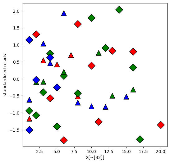
Replot the residuals
[18]:
resid = interM_lm32.get_influence().summary_frame()["standard_resid"]

plt.figure(figsize=(6, 6))
resid = resid.reindex(X.index)
for values, group in factor_groups:
    i, j = values
    idx = group.index
    plt.scatter(
        X.loc[idx],
        resid.loc[idx],
        marker=symbols[j],
        color=colors[i - 1],
        s=144,
        edgecolors="black",
    )
plt.xlabel("X[~[32]]")
plt.ylabel("standardized resids")
[18]:
Text(0, 0.5, 'standardized resids')
Plot the fitted values
[19]:
lm_final = ols("S ~ X + C(E)*C(M)", data=salary_table.drop([drop_idx])).fit()
mf = lm_final.model.data.orig_exog
lstyle = ["-", "--"]

plt.figure(figsize=(6, 6))
for values, group in factor_groups:
    i, j = values
    idx = group.index
    plt.scatter(
        X[idx],
        S[idx],
        marker=symbols[j],
        color=colors[i - 1],
        s=144,
        edgecolors="black",
    )
    # drop NA because there is no idx 32 in the final model
    fv = lm_final.fittedvalues.reindex(idx).dropna()
    x = mf.X.reindex(idx).dropna()
    plt.plot(x, fv, ls=lstyle[j], color=colors[i - 1])
plt.xlabel("Experience")
plt.ylabel("Salary")
[19]:
Text(0, 0.5, 'Salary')
From our first look at the data, the difference between Master’s and PhD in the management group is different than in the non-management group. This is an interaction between the two qualitative variables management,M and education,E. We can visualize this by first removing the effect of experience, then plotting the means within each of the 6 groups using interaction.plot.
[20]:
U = S - X * interX_lm32.params["X"]

plt.figure(figsize=(6, 6))
interaction_plot(
    E, M, U, colors=["red", "blue"], markers=["^", "D"], markersize=10, ax=plt.gca()
)
[20]:

Ethnic Employment Data
[21]:
url = "https://raw.githubusercontent.com/statsmodels/smdatasets/main/data/anova/jobtest/jobtest.table"
jobtest_table = pd.read_csv(download_file(url), sep="\t")

factor_group = jobtest_table.groupby(["ETHN"])

fig, ax = plt.subplots(figsize=(6, 6))
colors = ["purple", "green"]
markers = ["o", "v"]
for factor, group in factor_group:
    factor_id = np.squeeze(factor)
    ax.scatter(
        group["TEST"],
        group["JPERF"],
        color=colors[factor_id],
        marker=markers[factor_id],
        s=12**2,
    )
ax.set_xlabel("TEST")
ax.set_ylabel("JPERF")
[21]:
Text(0, 0.5, 'JPERF')
[22]:
min_lm = ols("JPERF ~ TEST", data=jobtest_table).fit()
print(min_lm.summary())
                            OLS Regression Results
==============================================================================
Dep. Variable:                  JPERF   R-squared:                       0.517
Model:                            OLS   Adj. R-squared:                  0.490
Method:                 Least Squares   F-statistic:                     19.25
Date:                Fri, 05 Dec 2025   Prob (F-statistic):           0.000356
Time:                        18:15:24   Log-Likelihood:                -36.614
No. Observations:                  20   AIC:                             77.23
Df Residuals:                      18   BIC:                             79.22
Df Model:                           1
Covariance Type:            nonrobust
==============================================================================
                 coef    std err          t      P>|t|      [0.025      0.975]
------------------------------------------------------------------------------
Intercept      1.0350      0.868      1.192      0.249      -0.789       2.859
TEST           2.3605      0.538      4.387      0.000       1.230       3.491
==============================================================================
Omnibus:                        0.324   Durbin-Watson:                   2.896
Prob(Omnibus):                  0.850   Jarque-Bera (JB):                0.483
Skew:                          -0.186   Prob(JB):                        0.785
Kurtosis:                       2.336   Cond. No.                         5.26
==============================================================================

Notes:
[1] Standard Errors assume that the covariance matrix of the errors is correctly specified.
[23]:
fig, ax = plt.subplots(figsize=(6, 6))
for factor, group in factor_group:
factor_id = np.squeeze(factor)
ax.scatter(
group["TEST"],
group["JPERF"],
color=colors[factor_id],
marker=markers[factor_id],
s=12**2,
)
ax.set_xlabel("TEST")
ax.set_ylabel("JPERF")
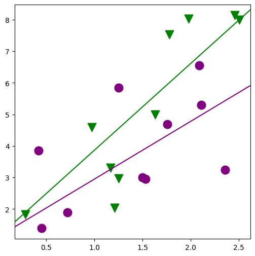
fig = abline_plot(model_results=min_lm, ax=ax)
[24]:
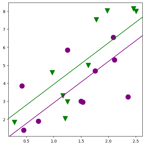
min_lm2 = ols("JPERF ~ TEST + TEST:ETHN", data=jobtest_table).fit()

print(min_lm2.summary())
                            OLS Regression Results
==============================================================================
Dep. Variable:                  JPERF   R-squared:                       0.632
Model:                            OLS   Adj. R-squared:                  0.589
Method:                 Least Squares   F-statistic:                     14.59
Date:                Fri, 05 Dec 2025   Prob (F-statistic):           0.000204
Time:                        18:15:24   Log-Likelihood:                -33.891
No. Observations:                  20   AIC:                             73.78
Df Residuals:                      17   BIC:                             76.77
Df Model:                           2
Covariance Type:            nonrobust
==============================================================================
                 coef    std err          t      P>|t|      [0.025      0.975]
------------------------------------------------------------------------------
Intercept      1.1211      0.780      1.437      0.169      -0.525       2.768
TEST           1.8276      0.536      3.412      0.003       0.698       2.958
TEST:ETHN      0.9161      0.397      2.306      0.034       0.078       1.754
==============================================================================
Omnibus:                        0.388   Durbin-Watson:                   3.008
Prob(Omnibus):                  0.823   Jarque-Bera (JB):                0.514
Skew:                           0.050   Prob(JB):                        0.773
Kurtosis:                       2.221   Cond. No.                         5.96
==============================================================================

Notes:
[1] Standard Errors assume that the covariance matrix of the errors is correctly specified.
[25]:
fig, ax = plt.subplots(figsize=(6, 6))
for factor, group in factor_group:
    factor_id = np.squeeze(factor)
    ax.scatter(
        group["TEST"],
        group["JPERF"],
        color=colors[factor_id],
        marker=markers[factor_id],
        s=12**2,
    )

fig = abline_plot(
    intercept=min_lm2.params["Intercept"],
    slope=min_lm2.params["TEST"],
    ax=ax,
    color="purple",
)
fig = abline_plot(
    intercept=min_lm2.params["Intercept"],
    slope=min_lm2.params["TEST"] + min_lm2.params["TEST:ETHN"],
    ax=ax,
    color="green",
)
[26]:
min_lm3 = ols("JPERF ~ TEST + ETHN", data=jobtest_table).fit()
print(min_lm3.summary())
                            OLS Regression Results
==============================================================================
Dep. Variable:                  JPERF   R-squared:                       0.572
Model:                            OLS   Adj. R-squared:                  0.522
Method:                 Least Squares   F-statistic:                     11.38
Date:                Fri, 05 Dec 2025   Prob (F-statistic):           0.000731
Time:                        18:15:24   Log-Likelihood:                -35.390
No. Observations:                  20   AIC:                             76.78
Df Residuals:                      17   BIC:                             79.77
Df Model:                           2
Covariance Type:            nonrobust
==============================================================================
                 coef    std err          t      P>|t|      [0.025      0.975]
------------------------------------------------------------------------------
Intercept      0.6120      0.887      0.690      0.500      -1.260       2.483
TEST           2.2988      0.522      4.400      0.000       1.197       3.401
ETHN           1.0276      0.691      1.487      0.155      -0.430       2.485
==============================================================================
Omnibus:                        0.251   Durbin-Watson:                   3.028
Prob(Omnibus):                  0.882   Jarque-Bera (JB):                0.437
Skew:                          -0.059   Prob(JB):                        0.804
Kurtosis:                       2.286   Cond. No.                         5.72
==============================================================================

Notes:
[1] Standard Errors assume that the covariance matrix of the errors is correctly specified.
[27]:
fig, ax = plt.subplots(figsize=(6, 6))
for factor, group in factor_group:
    factor_id = np.squeeze(factor)
    ax.scatter(
        group["TEST"],
        group["JPERF"],
        color=colors[factor_id],
        marker=markers[factor_id],
        s=12**2,
    )

fig = abline_plot(
    intercept=min_lm3.params["Intercept"],
    slope=min_lm3.params["TEST"],
    ax=ax,
    color="purple",
)
fig = abline_plot(
    intercept=min_lm3.params["Intercept"] + min_lm3.params["ETHN"],
    slope=min_lm3.params["TEST"],
    ax=ax,
    color="green",
)
[28]:
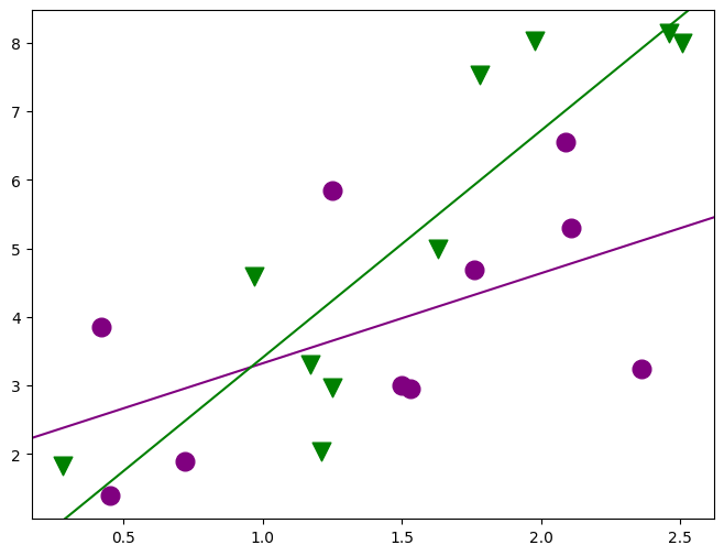
min_lm4 = ols("JPERF ~ TEST * ETHN", data=jobtest_table).fit()
print(min_lm4.summary())
                            OLS Regression Results
==============================================================================
Dep. Variable:                  JPERF   R-squared:                       0.664
Model:                            OLS   Adj. R-squared:                  0.601
Method:                 Least Squares   F-statistic:                     10.55
Date:                Fri, 05 Dec 2025   Prob (F-statistic):           0.000451
Time:                        18:15:25   Log-Likelihood:                -32.971
No. Observations:                  20   AIC:                             73.94
Df Residuals:                      16   BIC:                             77.92
Df Model:                           3
Covariance Type:            nonrobust
==============================================================================
                 coef    std err          t      P>|t|      [0.025      0.975]
------------------------------------------------------------------------------
Intercept      2.0103      1.050      1.914      0.074      -0.216       4.236
TEST           1.3134      0.670      1.959      0.068      -0.108       2.735
ETHN          -1.9132      1.540     -1.242      0.232      -5.179       1.352
TEST:ETHN      1.9975      0.954      2.093      0.053      -0.026       4.021
==============================================================================
Omnibus:                        3.377   Durbin-Watson:                   3.015
Prob(Omnibus):                  0.185   Jarque-Bera (JB):                1.330
Skew:                           0.120   Prob(JB):                        0.514
Kurtosis:                       1.760   Cond. No.                         13.8
==============================================================================

Notes:
[1] Standard Errors assume that the covariance matrix of the errors is correctly specified.
[29]:
fig, ax = plt.subplots(figsize=(8, 6))
for factor, group in factor_group:
    factor_id = np.squeeze(factor)
    ax.scatter(
        group["TEST"],
        group["JPERF"],
        color=colors[factor_id],
        marker=markers[factor_id],
        s=12**2,
    )

fig = abline_plot(
    intercept=min_lm4.params["Intercept"],
    slope=min_lm4.params["TEST"],
    ax=ax,
    color="purple",
)
fig = abline_plot(
    intercept=min_lm4.params["Intercept"] + min_lm4.params["ETHN"],
    slope=min_lm4.params["TEST"] + min_lm4.params["TEST:ETHN"],
    ax=ax,
    color="green",
)
[30]:
# is there any effect of ETHN on slope or intercept?
table5 = anova_lm(min_lm, min_lm4)
print(table5)
   df_resid        ssr  df_diff    ss_diff         F    Pr(>F)
0      18.0  45.568297      0.0        NaN       NaN       NaN
1      16.0  31.655473      2.0  13.912824  3.516061  0.054236
[31]:
# is there any effect of ETHN on intercept
table6 = anova_lm(min_lm, min_lm3)
print(table6)
   df_resid        ssr  df_diff   ss_diff         F    Pr(>F)
0      18.0  45.568297      0.0       NaN       NaN       NaN
1      17.0  40.321546      1.0  5.246751  2.212087  0.155246
[32]:
# is there any effect of ETHN on slope
table7 = anova_lm(min_lm, min_lm2)
print(table7)
   df_resid        ssr  df_diff    ss_diff         F    Pr(>F)
0      18.0  45.568297      0.0        NaN       NaN       NaN
1      17.0  34.707653      1.0  10.860644  5.319603  0.033949
[33]:
# is it just the slope or both?
table8 = anova_lm(min_lm2, min_lm4)
print(table8)
   df_resid        ssr  df_diff  ss_diff         F    Pr(>F)
0      17.0  34.707653      0.0      NaN       NaN       NaN
1      16.0  31.655473      1.0  3.05218  1.542699  0.232115
One-way ANOVA
[34]:
url = "https://raw.githubusercontent.com/statsmodels/smdatasets/main/data/anova/rehab/rehab.csv"
rehab_table = pd.read_csv(download_file(url))
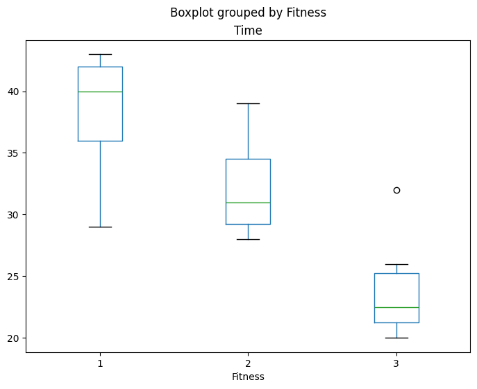
fig, ax = plt.subplots(figsize=(8, 6))
fig = rehab_table.boxplot("Time", "Fitness", ax=ax, grid=False)
[35]:
rehab_lm = ols("Time ~ C(Fitness)", data=rehab_table).fit()
table9 = anova_lm(rehab_lm)
print(table9)

print(rehab_lm.model.data.orig_exog)
              df  sum_sq     mean_sq          F    PR(>F)
C(Fitness)   2.0   672.0  336.000000  16.961538  0.000041
Residual    21.0   416.0   19.809524        NaN       NaN
    Intercept  C(Fitness)[T.2]  C(Fitness)[T.3]
0         1.0              0.0              0.0
1         1.0              0.0              0.0
2         1.0              0.0              0.0
3         1.0              0.0              0.0
4         1.0              0.0              0.0
5         1.0              0.0              0.0
6         1.0              0.0              0.0
7         1.0              0.0              0.0
8         1.0              1.0              0.0
9         1.0              1.0              0.0
10        1.0              1.0              0.0
11        1.0              1.0              0.0
12        1.0              1.0              0.0
13        1.0              1.0              0.0
14        1.0              1.0              0.0
15        1.0              1.0              0.0
16        1.0              1.0              0.0
17        1.0              1.0              0.0
18        1.0              0.0              1.0
19        1.0              0.0              1.0
20        1.0              0.0              1.0
21        1.0              0.0              1.0
22        1.0              0.0              1.0
23        1.0              0.0              1.0
[36]:
print(rehab_lm.summary())
                            OLS Regression Results
==============================================================================
Dep. Variable:                   Time   R-squared:                       0.618
Model:                            OLS   Adj. R-squared:                  0.581
Method:                 Least Squares   F-statistic:                     16.96
Date:                Fri, 05 Dec 2025   Prob (F-statistic):           4.13e-05
Time:                        18:15:26   Log-Likelihood:                -68.286
No. Observations:                  24   AIC:                             142.6
Df Residuals:                      21   BIC:                             146.1
Df Model:                           2
Covariance Type:            nonrobust
===================================================================================
                      coef    std err          t      P>|t|      [0.025      0.975]
-----------------------------------------------------------------------------------
Intercept          38.0000      1.574     24.149      0.000      34.728      41.272
C(Fitness)[T.2]    -6.0000      2.111     -2.842      0.010     -10.390      -1.610
C(Fitness)[T.3]   -14.0000      2.404     -5.824      0.000     -18.999      -9.001
==============================================================================
Omnibus:                        0.163   Durbin-Watson:                   2.209
Prob(Omnibus):                  0.922   Jarque-Bera (JB):                0.211
Skew:                          -0.163   Prob(JB):                        0.900
Kurtosis:                       2.675   Cond. No.                         3.80
==============================================================================

Notes:
[1] Standard Errors assume that the covariance matrix of the errors is correctly specified.
Two-way ANOVA
[37]:
url = "https://raw.githubusercontent.com/statsmodels/smdatasets/main/data/anova/kidney/kidney.table"
kidney_table = pd.read_csv(download_file(url), sep=r"\s+", engine="python")
Explore the dataset
[38]:
kidney_table.head(10)
[38]:
| Days | Duration | Weight | ID | |
|---|---|---|---|---|
| 0 | 0.0 | 1 | 1 | 1 |
| 1 | 2.0 | 1 | 1 | 2 |
| 2 | 1.0 | 1 | 1 | 3 |
| 3 | 3.0 | 1 | 1 | 4 |
| 4 | 0.0 | 1 | 1 | 5 |
| 5 | 2.0 | 1 | 1 | 6 |
| 6 | 0.0 | 1 | 1 | 7 |
| 7 | 5.0 | 1 | 1 | 8 |
| 8 | 6.0 | 1 | 1 | 9 |
| 9 | 8.0 | 1 | 1 | 10 |
Balanced panel
[39]:
kt = kidney_table
plt.figure(figsize=(8, 6))
fig = interaction_plot(
    kt["Weight"],
    kt["Duration"],
    np.log(kt["Days"] + 1),
    colors=["red", "blue"],
    markers=["D", "^"],
    ms=10,
    ax=plt.gca(),
)
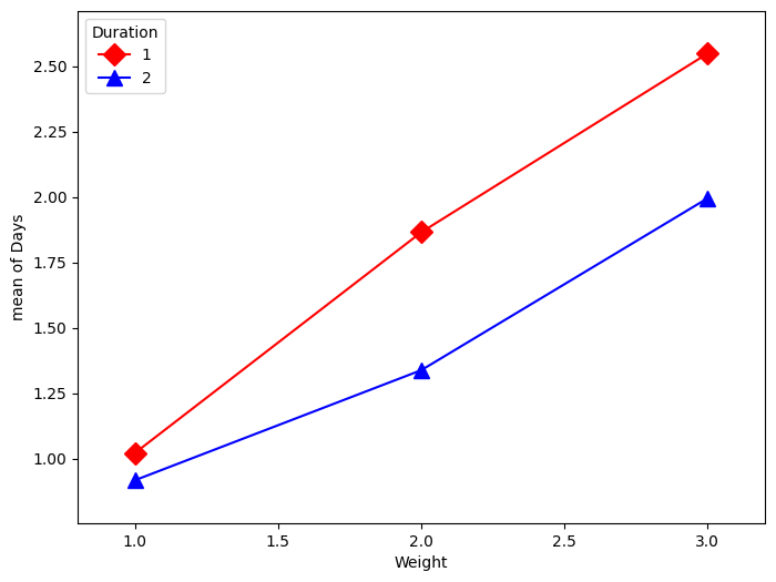
You have things available in the calling namespace available in the formula evaluation namespace
[40]:
kidney_lm = ols("np.log(Days+1) ~ C(Duration) * C(Weight)", data=kt).fit()

table10 = anova_lm(kidney_lm)

print(
    anova_lm(ols("np.log(Days+1) ~ C(Duration) + C(Weight)", data=kt).fit(), kidney_lm)
)
print(
    anova_lm(
        ols("np.log(Days+1) ~ C(Duration)", data=kt).fit(),
        ols("np.log(Days+1) ~ C(Duration) + C(Weight, Sum)", data=kt).fit(),
    )
)
print(
    anova_lm(
        ols("np.log(Days+1) ~ C(Weight)", data=kt).fit(),
        ols("np.log(Days+1) ~ C(Duration) + C(Weight, Sum)", data=kt).fit(),
    )
)
   df_resid        ssr  df_diff   ss_diff        F    Pr(>F)
0      56.0  29.624856      0.0       NaN      NaN       NaN
1      54.0  28.989198      2.0  0.635658  0.59204  0.556748
   df_resid        ssr  df_diff    ss_diff          F    Pr(>F)
0      58.0  46.596147      0.0        NaN        NaN       NaN
1      56.0  29.624856      2.0  16.971291  16.040454  0.000003
   df_resid        ssr  df_diff   ss_diff         F   Pr(>F)
0      57.0  31.964549      0.0       NaN       NaN      NaN
1      56.0  29.624856      1.0  2.339693  4.422732  0.03997
Sum of squares
Illustrates the use of different types of sums of squares (I,II,II) and how the Sum contrast can be used to produce the same output between the 3.
Types I and II are equivalent under a balanced design.
Do not use Type III with non-orthogonal contrast - ie., Treatment
[41]:
sum_lm = ols("np.log(Days+1) ~ C(Duration, Sum) * C(Weight, Sum)", data=kt).fit()

print(anova_lm(sum_lm))
print(anova_lm(sum_lm, typ=2))
print(anova_lm(sum_lm, typ=3))
                                   df     sum_sq   mean_sq          F    PR(>F)
C(Duration, Sum)                  1.0   2.339693  2.339693   4.358293  0.041562
C(Weight, Sum)                    2.0  16.971291  8.485645  15.806745  0.000004
C(Duration, Sum):C(Weight, Sum)   2.0   0.635658  0.317829   0.592040  0.556748
Residual                         54.0  28.989198  0.536837        NaN       NaN
                                    sum_sq    df          F    PR(>F)
C(Duration, Sum)                  2.339693   1.0   4.358293  0.041562
C(Weight, Sum)                   16.971291   2.0  15.806745  0.000004
C(Duration, Sum):C(Weight, Sum)   0.635658   2.0   0.592040  0.556748
Residual                         28.989198  54.0        NaN       NaN
                                     sum_sq    df           F        PR(>F)
Intercept                        156.301830   1.0  291.153237  2.077589e-23
C(Duration, Sum)                   2.339693   1.0    4.358293  4.156170e-02
C(Weight, Sum)                    16.971291   2.0   15.806745  3.944502e-06
C(Duration, Sum):C(Weight, Sum)    0.635658   2.0    0.592040  5.567479e-01
Residual                          28.989198  54.0         NaN           NaN
[42]:
nosum_lm = ols(
    "np.log(Days+1) ~ C(Duration, Treatment) * C(Weight, Treatment)", data=kt
).fit()
print(anova_lm(nosum_lm))
print(anova_lm(nosum_lm, typ=2))
print(anova_lm(nosum_lm, typ=3))
                                               df     sum_sq   mean_sq          F    PR(>F)
C(Duration, Treatment)                        1.0   2.339693  2.339693   4.358293  0.041562
C(Weight, Treatment)                          2.0  16.971291  8.485645  15.806745  0.000004
C(Duration, Treatment):C(Weight, Treatment)   2.0   0.635658  0.317829   0.592040  0.556748
Residual                                     54.0  28.989198  0.536837        NaN       NaN
                                                sum_sq    df          F    PR(>F)
C(Duration, Treatment)                        2.339693   1.0   4.358293  0.041562
C(Weight, Treatment)                         16.971291   2.0  15.806745  0.000004
C(Duration, Treatment):C(Weight, Treatment)   0.635658   2.0   0.592040  0.556748
Residual                                     28.989198  54.0        NaN       NaN
                                                sum_sq    df          F    PR(>F)
Intercept                                    10.427596   1.0  19.424139  0.000050
C(Duration, Treatment)                        0.054293   1.0   0.101134  0.751699
C(Weight, Treatment)                         11.703387   2.0  10.900317  0.000106
C(Duration, Treatment):C(Weight, Treatment)   0.635658   2.0   0.592040  0.556748
Residual                                     28.989198  54.0        NaN       NaN