Prediction (out of sample)
[1]:
%matplotlib inline
[2]:
import numpy as np
import matplotlib.pyplot as plt

import statsmodels.api as sm

plt.rc("figure", figsize=(16, 8))
plt.rc("font", size=14)
Artificial data
[3]:
nsample = 50
sig = 0.25
x1 = np.linspace(0, 20, nsample)
X = np.column_stack((x1, np.sin(x1), (x1 - 5) ** 2))
X = sm.add_constant(X)
beta = [5.0, 0.5, 0.5, -0.02]
y_true = np.dot(X, beta)
y = y_true + sig * np.random.normal(size=nsample)
Estimation
[4]:
olsmod = sm.OLS(y, X)
olsres = olsmod.fit()
print(olsres.summary())
                            OLS Regression Results
==============================================================================
Dep. Variable:                      y   R-squared:                       0.979
Model:                            OLS   Adj. R-squared:                  0.977
Method:                 Least Squares   F-statistic:                     702.6
Date:                Fri, 12 Apr 2024   Prob (F-statistic):           2.06e-38
Time:                        16:02:49   Log-Likelihood:                -6.0264
No. Observations:                  50   AIC:                             20.05
Df Residuals:                      46   BIC:                             27.70
Df Model:                           3
Covariance Type:            nonrobust
==============================================================================
                 coef    std err          t      P>|t|      [0.025      0.975]
------------------------------------------------------------------------------
const          5.0160      0.097     51.712      0.000       4.821       5.211
x1             0.4983      0.015     33.309      0.000       0.468       0.528
x2             0.5523      0.059      9.391      0.000       0.434       0.671
x3            -0.0197      0.001    -15.017      0.000      -0.022      -0.017
==============================================================================
Omnibus:                        3.556   Durbin-Watson:                   1.759
Prob(Omnibus):                  0.169   Jarque-Bera (JB):                1.938
Skew:                          -0.202   Prob(JB):                        0.379
Kurtosis:                       2.124   Cond. No.                         221.
==============================================================================

Notes:
[1] Standard Errors assume that the covariance matrix of the errors is correctly specified.
In-sample prediction
[5]:
ypred = olsres.predict(X)
print(ypred)
[ 4.52294204  5.02276451  5.47999809  5.86454335  6.1571636   6.35264542
  6.46065517  6.50415086  6.51561024  6.53169474  6.58722616  6.70946549
  6.91363407  7.20041269  7.55582982  7.95355704  8.35923472  8.73611726
  9.05111023  9.28020773  9.41243647  9.45165868  9.41593751  9.33456935
  9.24327048  9.17830903  9.17054618  9.24036578  9.39432535  9.62407868
  9.90774711 10.21351409 10.5048526  10.7465264  10.91037928 10.97996099
 10.95323002 10.84288901 10.67429771 10.48130647 10.30069471 10.16612819
 10.10262779 10.12245866 10.22311512 10.38773228 10.58785694 10.78812235
 10.95205887 11.04808585]
Create a new sample of explanatory variables Xnew, predict and plot
[6]:
x1n = np.linspace(20.5, 25, 10)
Xnew = np.column_stack((x1n, np.sin(x1n), (x1n - 5) ** 2))
Xnew = sm.add_constant(Xnew)
ynewpred = olsres.predict(Xnew)  # predict out of sample
print(ynewpred)
[11.04276416 10.89278875 10.61981841 10.27321077  9.91793788  9.61867873
  9.4239836   9.35438726  9.39738134  9.51047682]
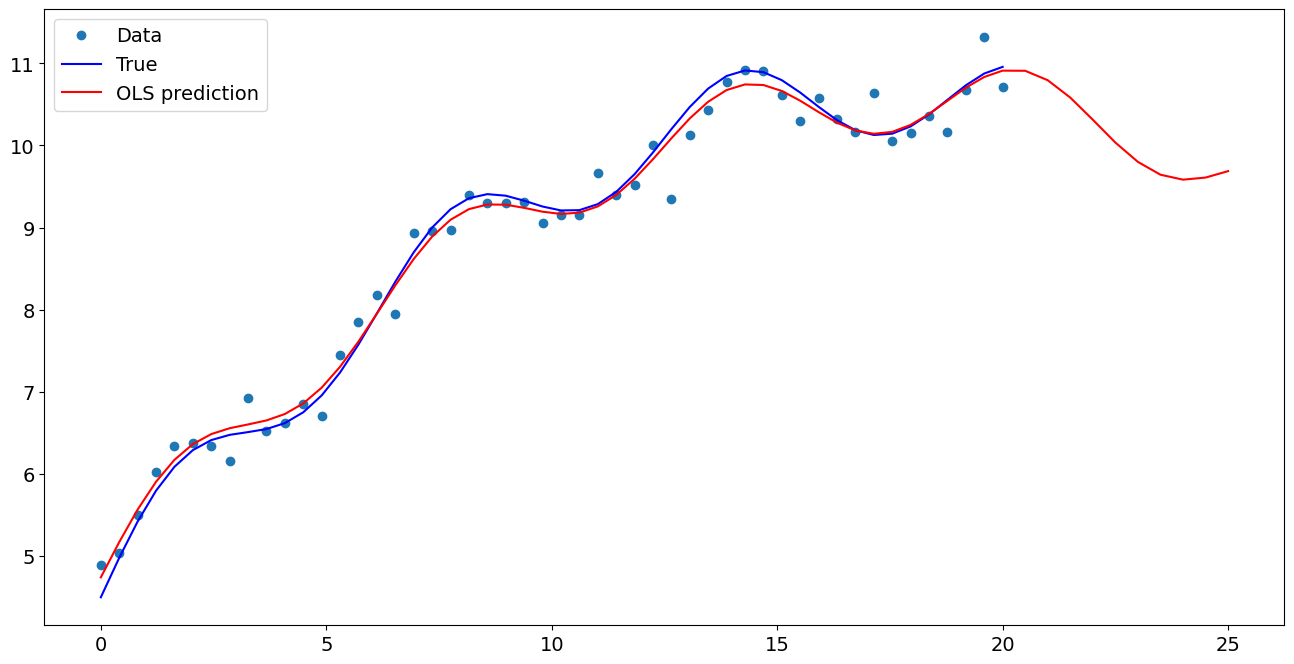
Plot comparison
[7]:
import matplotlib.pyplot as plt

fig, ax = plt.subplots()
ax.plot(x1, y, "o", label="Data")
ax.plot(x1, y_true, "b-", label="True")
ax.plot(np.hstack((x1, x1n)), np.hstack((ypred, ynewpred)), "r", label="OLS prediction")
ax.legend(loc="best")
[7]:
<matplotlib.legend.Legend at 0x7f4ec5eb0a90>
Predicting with Formulas
Using formulas can make both estimation and prediction a lot easier
[8]:
from statsmodels.formula.api import ols

data = {"x1": x1, "y": y}

res = ols("y ~ x1 + np.sin(x1) + I((x1-5)**2)", data=data).fit()
We use the I to indicate use of the Identity transform. Ie., we do not want any expansion magic from using **2
[9]:
res.params
[9]:
Intercept           5.016049
x1                  0.498289
np.sin(x1)          0.552292
I((x1 - 5) ** 2)   -0.019724
dtype: float64
Now we only have to pass the single variable and we get the transformed right-hand side variables automatically
[10]:
res.predict(exog=dict(x1=x1n))
[10]:
0    11.042764
1    10.892789
2    10.619818
3    10.273211
4     9.917938
5     9.618679
6     9.423984
7     9.354387
8     9.397381
9     9.510477
dtype: float64
Last update:
Apr 12, 2024