Autoregressive Moving Average (ARMA): Sunspots data¶

This notebook replicates the existing ARMA notebook using the statsmodels.tsa.statespace.SARIMAX class rather than the statsmodels.tsa.ARMA class.

[1]:

%matplotlib inline

[2]:

import numpy as np
from scipy import stats
import pandas as pd
import matplotlib.pyplot as plt

import statsmodels.api as sm

[3]:

from statsmodels.graphics.api import qqplot

Sunspots Data¶

[4]:

print(sm.datasets.sunspots.NOTE)

::

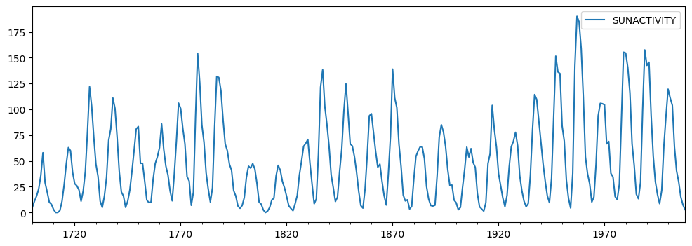
    Number of Observations - 309 (Annual 1700 - 2008)
    Number of Variables - 1
    Variable name definitions::

        SUNACTIVITY - Number of sunspots for each year

    The data file contains a 'YEAR' variable that is not returned by load.

[5]:

dta = sm.datasets.sunspots.load_pandas().data

[6]:

dta.index = pd.Index(pd.date_range("1700", end="2009", freq="A-DEC"))
del dta["YEAR"]

/tmp/ipykernel_5132/1301052817.py:1: FutureWarning: 'A-DEC' is deprecated and will be removed in a future version, please use 'YE-DEC' instead.
  dta.index = pd.Index(pd.date_range("1700", end="2009", freq="A-DEC"))

[7]:

dta.plot(figsize=(12,4));

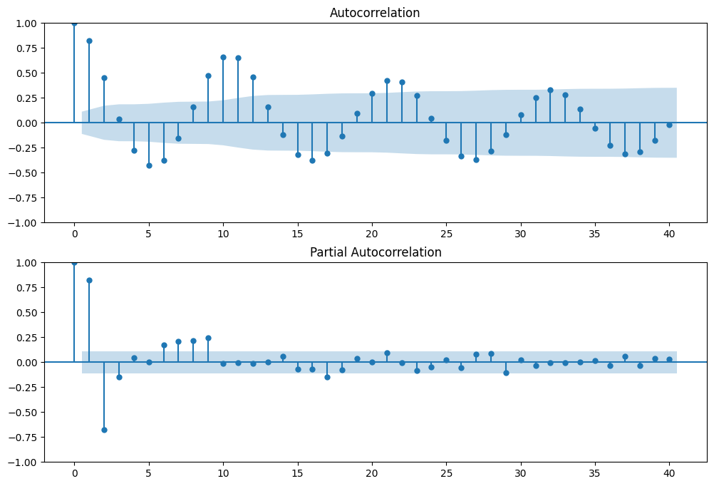
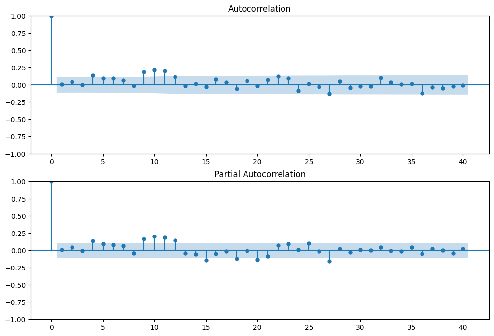
../../../_images/examples_notebooks_generated_statespace_arma_0_9_0.png

[8]:

fig = plt.figure(figsize=(12,8))
ax1 = fig.add_subplot(211)
fig = sm.graphics.tsa.plot_acf(dta.values.squeeze(), lags=40, ax=ax1)
ax2 = fig.add_subplot(212)
fig = sm.graphics.tsa.plot_pacf(dta, lags=40, ax=ax2)

../../../_images/examples_notebooks_generated_statespace_arma_0_10_0.png

[9]:

arma_mod20 = sm.tsa.statespace.SARIMAX(dta, order=(2,0,0), trend='c').fit(disp=False)
print(arma_mod20.params)

intercept     14.793947
ar.L1          1.390659
ar.L2         -0.688568
sigma2       274.761104
dtype: float64

[10]:

arma_mod30 = sm.tsa.statespace.SARIMAX(dta, order=(3,0,0), trend='c').fit(disp=False)

[11]:

print(arma_mod20.aic, arma_mod20.bic, arma_mod20.hqic)

2622.636338141591 2637.5697032491817 2628.606725986837

[12]:

print(arma_mod30.params)

intercept     16.762205
ar.L1          1.300810
ar.L2         -0.508122
ar.L3         -0.129612
sigma2       270.102651
dtype: float64

[13]:

print(arma_mod30.aic, arma_mod30.bic, arma_mod30.hqic)

2619.4036296633913 2638.07033604788 2626.8666144699487

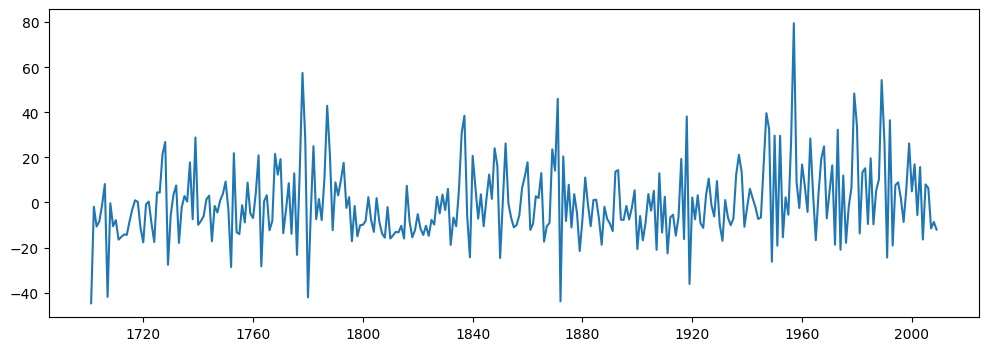
Does our model obey the theory?

[14]:

sm.stats.durbin_watson(arma_mod30.resid)

[14]:

1.9564844817900373

[15]:

fig = plt.figure(figsize=(12,4))
ax = fig.add_subplot(111)
ax = plt.plot(arma_mod30.resid)

../../../_images/examples_notebooks_generated_statespace_arma_0_18_0.png

[16]:

resid = arma_mod30.resid

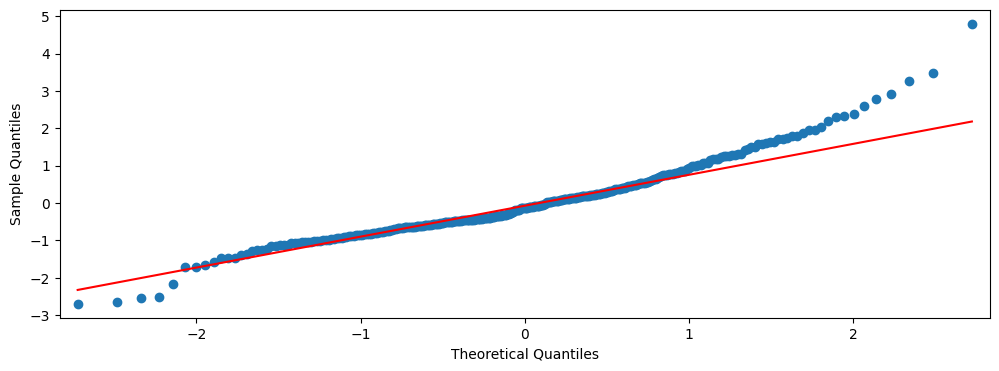
[17]:

stats.normaltest(resid)

[17]:

NormaltestResult(statistic=49.84700631937409, pvalue=1.499201845134695e-11)

[18]:

fig = plt.figure(figsize=(12,4))
ax = fig.add_subplot(111)
fig = qqplot(resid, line='q', ax=ax, fit=True)

../../../_images/examples_notebooks_generated_statespace_arma_0_21_0.png

[19]:

fig = plt.figure(figsize=(12,8))
ax1 = fig.add_subplot(211)
fig = sm.graphics.tsa.plot_acf(resid, lags=40, ax=ax1)
ax2 = fig.add_subplot(212)
fig = sm.graphics.tsa.plot_pacf(resid, lags=40, ax=ax2)

../../../_images/examples_notebooks_generated_statespace_arma_0_22_0.png

[20]:

r,q,p = sm.tsa.acf(resid, fft=True, qstat=True)
data = np.c_[r[1:], q, p]
index = pd.Index(range(1,q.shape[0]+1), name="lag")
table = pd.DataFrame(data, columns=["AC", "Q", "Prob(>Q)"], index=index)
print(table)

           AC          Q      Prob(>Q)
lag
1    0.009176   0.026273  8.712350e-01
2    0.041820   0.573727  7.506142e-01
3   -0.001342   0.574292  9.022915e-01
4    0.136064   6.407488  1.707135e-01
5    0.092433   9.108334  1.048203e-01
6    0.091919  11.788018  6.686842e-02
7    0.068735  13.291375  6.531941e-02
8   -0.015021  13.363411  9.994248e-02
9    0.187599  24.636916  3.400197e-03
10   0.213724  39.317881  2.233182e-05
11   0.201092  52.358270  2.347759e-07
12   0.117192  56.802110  8.581666e-08
13  -0.014051  56.866210  1.895534e-07
14   0.015394  56.943403  4.001105e-07
15  -0.024986  57.147464  7.747084e-07
16   0.080892  59.293627  6.880520e-07
17   0.041120  59.850085  1.112486e-06
18  -0.052030  60.744064  1.550379e-06
19   0.062500  62.038495  1.833802e-06
20  -0.010292  62.073718  3.385223e-06
21   0.074467  63.924063  3.196544e-06
22   0.124962  69.152771  8.984833e-07
23   0.093170  72.069532  5.802915e-07
24  -0.082149  74.345042  4.715786e-07

This indicates a lack of fit.

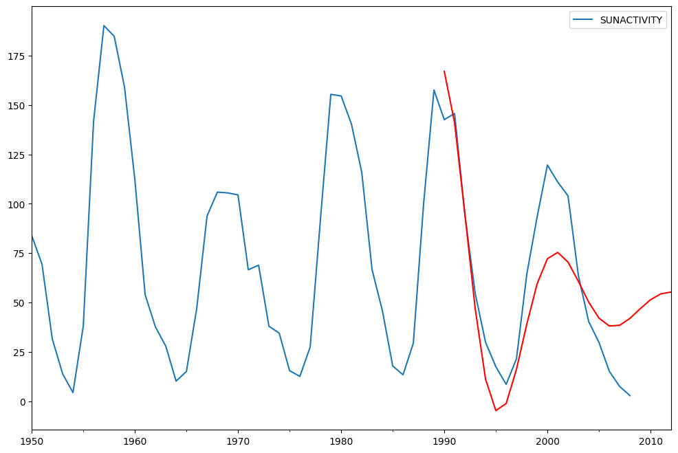
In-sample dynamic prediction. How good does our model do?

[21]:

predict_sunspots = arma_mod30.predict(start='1990', end='2012', dynamic=True)

[22]:

fig, ax = plt.subplots(figsize=(12, 8))
dta.loc['1950':].plot(ax=ax)
predict_sunspots.plot(ax=ax, style='r');

../../../_images/examples_notebooks_generated_statespace_arma_0_27_0.png

[23]:

def mean_forecast_err(y, yhat):
    return y.sub(yhat).mean()

[24]:

mean_forecast_err(dta.SUNACTIVITY, predict_sunspots)

[24]:

5.635549988344077

Last update: Apr 16, 2024