statsmodels.tsa.seasonal.STL¶

class statsmodels.tsa.seasonal.STL(endog, period=None, seasonal=7, trend=None, low_pass=None, seasonal_deg=1, trend_deg=1, low_pass_deg=1, robust=False, seasonal_jump=1, trend_jump=1, low_pass_jump=1)¶

Season-Trend decomposition using LOESS.

Parameters:¶

endogarray_like

Data to be decomposed. Must be squeezable to 1-d.

period{int, None}, optional

Periodicity of the sequence. If None and endog is a pandas Series or DataFrame, attempts to determine from endog. If endog is a ndarray, period must be provided.

seasonalint, optional

Length of the seasonal smoother. Must be an odd integer, and should normally be >= 7 (default).

trend{int, None}, optional

Length of the trend smoother. Must be an odd integer. If not provided uses the smallest odd integer greater than 1.5 * period / (1 - 1.5 / seasonal), following the suggestion in the original implementation.

low_pass{int, None}, optional

Length of the low-pass filter. Must be an odd integer >=3. If not provided, uses the smallest odd integer > period.

seasonal_degint, optional

Degree of seasonal LOESS. 0 (constant) or 1 (constant and trend).

trend_degint, optional

Degree of trend LOESS. 0 (constant) or 1 (constant and trend).

low_pass_degint, optional

Degree of low pass LOESS. 0 (constant) or 1 (constant and trend).

robustbool, optional

Flag indicating whether to use a weighted version that is robust to some forms of outliers.

seasonal_jumpint, optional

Positive integer determining the linear interpolation step. If larger than 1, the LOESS is used every seasonal_jump points and linear interpolation is between fitted points. Higher values reduce estimation time.

trend_jumpint, optional

Positive integer determining the linear interpolation step. If larger than 1, the LOESS is used every trend_jump points and values between the two are linearly interpolated. Higher values reduce estimation time.

low_pass_jumpint, optional

Positive integer determining the linear interpolation step. If larger than 1, the LOESS is used every low_pass_jump points and values between the two are linearly interpolated. Higher values reduce estimation time.

See also

statsmodels.tsa.seasonal.DecomposeResult

statsmodels.tsa.seasonal.seasonal_decompose

Notes

Derived from the NETLIB fortran written by [1]. The original code contains a bug that appears in the determination of the median that is used in the robust weighting. This version matches the fixed version that uses a correct partitioned sort to determine the median.

See the notebook Seasonal Decomposition for an overview.

References

[1]

R. B. Cleveland, W. S. Cleveland, J.E. McRae, and I. Terpenning (1990) STL: A Seasonal-Trend Decomposition Procedure Based on LOESS. Journal of Official Statistics, 6, 3-73.

Examples

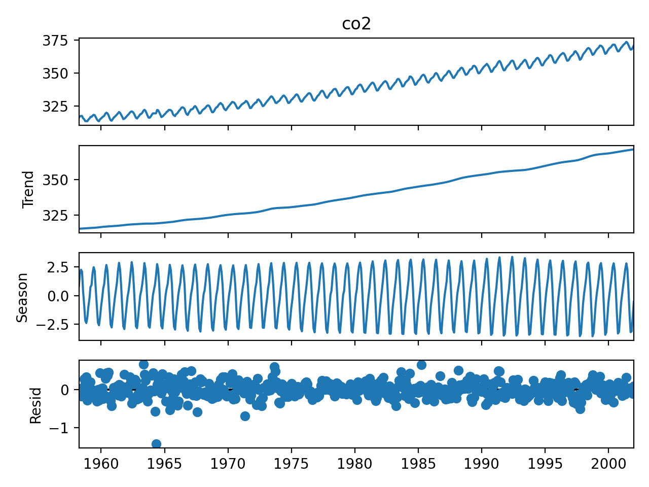
The original example uses STL to decompose CO2 data into level, season and a residual.

Start by aggregating to monthly, and filling any missing values

>>> from statsmodels.datasets import co2
>>> import matplotlib.pyplot as plt
>>> from pandas.plotting import register_matplotlib_converters
>>> register_matplotlib_converters()
>>> data = co2.load(True).data
>>> data = data.resample('M').mean().ffill()

The period (12) is automatically detected from the data’s frequency (‘M’).

>>> from statsmodels.tsa.seasonal import STL
>>> res = STL(data).fit()
>>> res.plot()
>>> plt.show()

(Source code, png, hires.png, pdf)

Attributes:¶

config

The parameters used in the model.

period

The period length of the time series

Methods

fit([inner_iter, outer_iter])

Estimate season, trend and residuals components.

Properties

config	The parameters used in the model.
period	The period length of the time series