Autoregressive Moving Average (ARMA): Artificial data
[1]:
%matplotlib inline
[2]:
import numpy as np
import pandas as pd

from statsmodels.graphics.tsaplots import plot_predict
from statsmodels.tsa.arima_process import arma_generate_sample
from statsmodels.tsa.arima.model import ARIMA

np.random.seed(12345)
Generate some data from an ARMA process:
[3]:
arparams = np.array([0.75, -0.25])
maparams = np.array([0.65, 0.35])
The conventions of the arma_generate function require that we specify a 1 for the zero-lag of the AR and MA parameters and that the AR parameters be negated.
[4]:
arparams = np.r_[1, -arparams]
maparams = np.r_[1, maparams]
nobs = 250
y = arma_generate_sample(arparams, maparams, nobs)
Now, optionally, we can add some dates information. For this example, we’ll use a pandas time series.
[5]:
dates = pd.date_range("1980-1-1", freq="M", periods=nobs)
y = pd.Series(y, index=dates)
arma_mod = ARIMA(y, order=(2, 0, 2), trend="n")
arma_res = arma_mod.fit()
/tmp/ipykernel_4160/3761908329.py:1: FutureWarning: 'M' is deprecated and will be removed in a future version, please use 'ME' instead.
  dates = pd.date_range("1980-1-1", freq="M", periods=nobs)
[6]:
print(arma_res.summary())
                               SARIMAX Results
==============================================================================
Dep. Variable:                      y   No. Observations:                  250
Model:                 ARIMA(2, 0, 2)   Log Likelihood                -353.445
Date:                Fri, 19 Apr 2024   AIC                            716.891
Time:                        16:18:05   BIC                            734.498
Sample:                    01-31-1980   HQIC                           723.977
                         - 10-31-2000
Covariance Type:                  opg
==============================================================================
                 coef    std err          z      P>|z|      [0.025      0.975]
------------------------------------------------------------------------------
ar.L1          0.7905      0.142      5.566      0.000       0.512       1.069
ar.L2         -0.2314      0.124     -1.859      0.063      -0.475       0.013
ma.L1          0.7007      0.131      5.344      0.000       0.444       0.958
ma.L2          0.4061      0.097      4.177      0.000       0.216       0.597
sigma2         0.9801      0.093     10.514      0.000       0.797       1.163
===================================================================================
Ljung-Box (L1) (Q):                   0.00   Jarque-Bera (JB):                 0.29
Prob(Q):                              0.96   Prob(JB):                         0.86
Heteroskedasticity (H):               0.92   Skew:                             0.02
Prob(H) (two-sided):                  0.69   Kurtosis:                         2.84
===================================================================================

Warnings:
[1] Covariance matrix calculated using the outer product of gradients (complex-step).
[7]:
y.tail()
[7]:
2000-06-30    0.173211
2000-07-31   -0.048325
2000-08-31   -0.415804
2000-09-30    0.338725
2000-10-31    0.360838
Freq: ME, dtype: float64
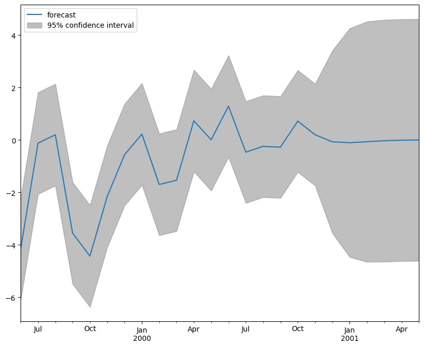
[8]:
import matplotlib.pyplot as plt

fig, ax = plt.subplots(figsize=(10, 8))
fig = plot_predict(arma_res, start="1999-06-30", end="2001-05-31", ax=ax)
legend = ax.legend(loc="upper left")
Last update:
Apr 19, 2024