statsmodels.graphics.tsaplots.plot_acf¶

statsmodels.graphics.tsaplots.plot_acf(x, ax=None, lags=None, *, alpha=0.05, use_vlines=True, adjusted=False, fft=False, missing='none', title='Autocorrelation', zero=True, auto_ylims=False, bartlett_confint=True, vlines_kwargs=None, **kwargs)[source]¶

Plot the autocorrelation function

Plots lags on the horizontal and the correlations on vertical axis.

Parameters:¶

xarray_like

Array of time-series values

axAxesSubplot, optional

If given, this subplot is used to plot in instead of a new figure being created.

lags{int, array_like}, optional

An int or array of lag values, used on horizontal axis. Uses np.arange(lags) when lags is an int. If not provided, lags=np.arange(len(corr)) is used.

alphascalar, optional

If a number is given, the confidence intervals for the given level are returned. For instance if alpha=.05, 95 % confidence intervals are returned where the standard deviation is computed according to Bartlett’s formula. If None, no confidence intervals are plotted.

use_vlinesbool, optional

If True, vertical lines and markers are plotted. If False, only markers are plotted. The default marker is ‘o’; it can be overridden with a marker kwarg.

adjustedbool

If True, then denominators for autocovariance are n-k, otherwise n

fftbool, optional

If True, computes the ACF via FFT.

missingstr, optional

A string in [‘none’, ‘raise’, ‘conservative’, ‘drop’] specifying how the NaNs are to be treated.

titlestr, optional

Title to place on plot. Default is ‘Autocorrelation’

zerobool, optional

Flag indicating whether to include the 0-lag autocorrelation. Default is True.

auto_ylimsbool, optional

If True, adjusts automatically the y-axis limits to ACF values.

bartlett_confintbool, default True

Confidence intervals for ACF values are generally placed at 2 standard errors around r_k. The formula used for standard error depends upon the situation. If the autocorrelations are being used to test for randomness of residuals as part of the ARIMA routine, the standard errors are determined assuming the residuals are white noise. The approximate formula for any lag is that standard error of each r_k = 1/sqrt(N). See section 9.4 of [1] for more details on the 1/sqrt(N) result. For more elementary discussion, see section 5.3.2 in [2]. For the ACF of raw data, the standard error at a lag k is found as if the right model was an MA(k-1). This allows the possible interpretation that if all autocorrelations past a certain lag are within the limits, the model might be an MA of order defined by the last significant autocorrelation. In this case, a moving average model is assumed for the data and the standard errors for the confidence intervals should be generated using Bartlett’s formula. For more details on Bartlett formula result, see section 7.2 in [1].

vlines_kwargsdict, optional

Optional dictionary of keyword arguments that are passed to vlines.

**kwargskwargs, optional

Optional keyword arguments that are directly passed on to the Matplotlib plot and axhline functions.

Returns:¶

Figure

If ax is None, the created figure. Otherwise the figure to which ax is connected.

See also

matplotlib.pyplot.xcorr

matplotlib.pyplot.acorr

Notes

Adapted from matplotlib’s xcorr.

Data are plotted as plot(lags, corr, **kwargs)

kwargs is used to pass matplotlib optional arguments to both the line tracing the autocorrelations and for the horizontal line at 0. These options must be valid for a Line2D object.

vlines_kwargs is used to pass additional optional arguments to the vertical lines connecting each autocorrelation to the axis. These options must be valid for a LineCollection object.

References

[1] Brockwell and Davis, 1987. Time Series Theory and Methods [2] Brockwell and Davis, 2010. Introduction to Time Series and Forecasting, 2nd edition.

Examples

>>> import pandas as pd
>>> import matplotlib.pyplot as plt
>>> import statsmodels.api as sm

>>> dta = sm.datasets.sunspots.load_pandas().data
>>> dta.index = pd.Index(sm.tsa.datetools.dates_from_range('1700', '2008'))
>>> del dta["YEAR"]
>>> sm.graphics.tsa.plot_acf(dta.values.squeeze(), lags=40)
>>> plt.show()

(Source code, png, hires.png, pdf)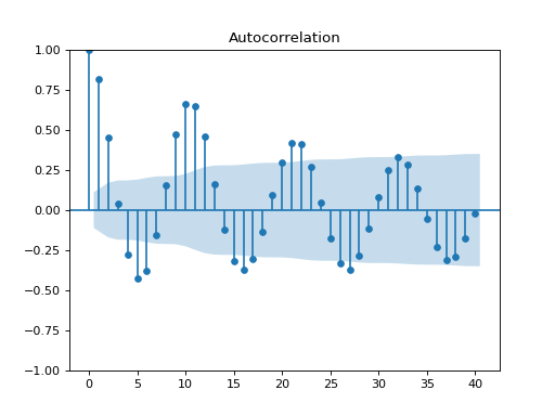