Meta-Analysis in statsmodels
Statsmodels include basic methods for meta-analysis. This notebook illustrates the current usage.
Status: The results have been verified against R meta and metafor packages. However, the API is still experimental and will still change. Some options for additional methods that are available in R meta and metafor are missing.
The support for meta-analysis has 3 parts:
effect size functions: this currently includes
effectsize_smdcomputes effect size and their standard errors for standardized mean difference,effectsize_2proportionscomputes effect sizes for comparing two independent proportions using risk difference, (log) risk ratio, (log) odds-ratio or arcsine square root transformationThe
combine_effectscomputes fixed and random effects estimate for the overall mean or effect. The returned results instance includes a forest plot function.helper functions to estimate the random effect variance, tau-squared
The estimate of the overall effect size in combine_effects can also be performed using WLS or GLM with var_weights.
Finally, the meta-analysis functions currently do not include the Mantel-Hanszel method. However, the fixed effects results can be computed directly using StratifiedTable as illustrated below.
[1]:
%matplotlib inline
[2]:
import numpy as np
import pandas as pd
from scipy import stats, optimize

from statsmodels.regression.linear_model import WLS
from statsmodels.genmod.generalized_linear_model import GLM

from statsmodels.stats.meta_analysis import (
    effectsize_smd,
    effectsize_2proportions,
    combine_effects,
    _fit_tau_iterative,
    _fit_tau_mm,
    _fit_tau_iter_mm,
)

# increase line length for pandas
pd.set_option("display.width", 100)
Example
[3]:
data = [
    ["Carroll", 94, 22, 60, 92, 20, 60],
    ["Grant", 98, 21, 65, 92, 22, 65],
    ["Peck", 98, 28, 40, 88, 26, 40],
    ["Donat", 94, 19, 200, 82, 17, 200],
    ["Stewart", 98, 21, 50, 88, 22, 45],
    ["Young", 96, 21, 85, 92, 22, 85],
]
colnames = ["study", "mean_t", "sd_t", "n_t", "mean_c", "sd_c", "n_c"]
rownames = [i[0] for i in data]
dframe1 = pd.DataFrame(data, columns=colnames)
rownames
[3]:
['Carroll', 'Grant', 'Peck', 'Donat', 'Stewart', 'Young']
[4]:
mean2, sd2, nobs2, mean1, sd1, nobs1 = np.asarray(
    dframe1[["mean_t", "sd_t", "n_t", "mean_c", "sd_c", "n_c"]]
).T
rownames = dframe1["study"]
rownames.tolist()
[4]:
['Carroll', 'Grant', 'Peck', 'Donat', 'Stewart', 'Young']
[5]:
np.array(nobs1 + nobs2)
[5]:
array([120, 130, 80, 400, 95, 170])
estimate effect size standardized mean difference
[6]:
eff, var_eff = effectsize_smd(mean2, sd2, nobs2, mean1, sd1, nobs1)
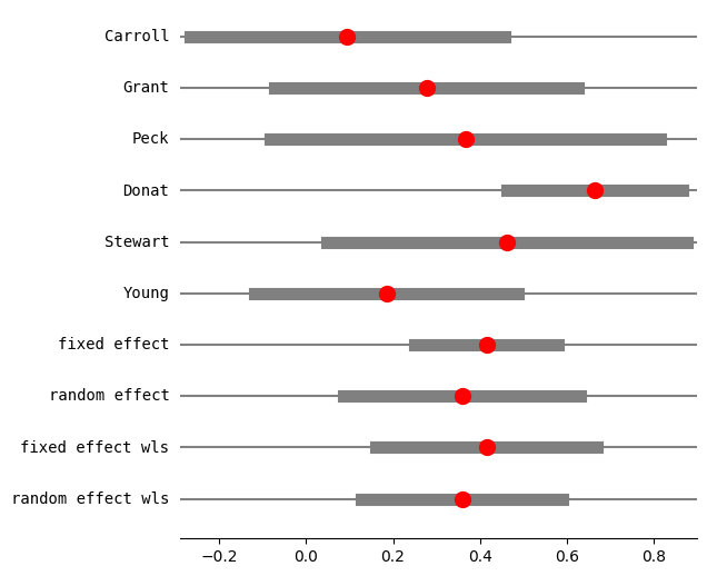
Using one-step chi2, DerSimonian-Laird estimate for random effects variance tau
Method option for random effect method_re="chi2" or method_re="dl", both names are accepted. This is commonly referred to as the DerSimonian-Laird method, it is based on a moment estimator based on pearson chi2 from the fixed effects estimate.
[7]:
res3 = combine_effects(eff, var_eff, method_re="chi2", use_t=True, row_names=rownames)
# TODO: we still need better information about conf_int of individual samples
# We don't have enough information in the model for individual confidence intervals
# if those are not based on normal distribution.
res3.conf_int_samples(nobs=np.array(nobs1 + nobs2))
print(res3.summary_frame())
                        eff    sd_eff    ci_low    ci_upp      w_fe      w_re
Carroll            0.094524  0.182680 -0.267199  0.456248  0.123885  0.157529
Grant              0.277356  0.176279 -0.071416  0.626129  0.133045  0.162828
Peck               0.366546  0.225573 -0.082446  0.815538  0.081250  0.126223
Donat              0.664385  0.102748  0.462389  0.866381  0.391606  0.232734
Stewart            0.461808  0.208310  0.048203  0.875413  0.095275  0.137949
Young              0.185165  0.153729 -0.118312  0.488641  0.174939  0.182736
fixed effect       0.414961  0.064298  0.249677  0.580245  1.000000       NaN
random effect      0.358486  0.105462  0.087388  0.629583       NaN  1.000000
fixed effect wls   0.414961  0.099237  0.159864  0.670058  1.000000       NaN
random effect wls  0.358486  0.090328  0.126290  0.590682       NaN  1.000000
[8]:
res3.cache_ci
[8]:
{(0.05,
  True): (array([-0.26719942, -0.07141628, -0.08244568,  0.46238908,  0.04820269,
         -0.1183121 ]), array([0.45624817, 0.62612908, 0.81553838, 0.86638112, 0.87541326,
         0.48864139]))}
[9]:
res3.method_re
[9]:
'chi2'
[10]:
fig = res3.plot_forest()
fig.set_figheight(6)
fig.set_figwidth(6)
[11]:
res3 = combine_effects(eff, var_eff, method_re="chi2", use_t=False, row_names=rownames)
# TODO: we still need better information about conf_int of individual samples
# We don't have enough information in the model for individual confidence intervals
# if those are not based on normal distribution.
res3.conf_int_samples(nobs=np.array(nobs1 + nobs2))
print(res3.summary_frame())
                        eff    sd_eff    ci_low    ci_upp      w_fe      w_re
Carroll            0.094524  0.182680 -0.263521  0.452570  0.123885  0.157529
Grant              0.277356  0.176279 -0.068144  0.622857  0.133045  0.162828
Peck               0.366546  0.225573 -0.075569  0.808662  0.081250  0.126223
Donat              0.664385  0.102748  0.463002  0.865768  0.391606  0.232734
Stewart            0.461808  0.208310  0.053527  0.870089  0.095275  0.137949
Young              0.185165  0.153729 -0.116139  0.486468  0.174939  0.182736
fixed effect       0.414961  0.064298  0.288939  0.540984  1.000000       NaN
random effect      0.358486  0.105462  0.151785  0.565187       NaN  1.000000
fixed effect wls   0.414961  0.099237  0.220460  0.609462  1.000000       NaN
random effect wls  0.358486  0.090328  0.181446  0.535526       NaN  1.000000
Using iterated, Paule-Mandel estimate for random effects variance tau
The method commonly referred to as Paule-Mandel estimate is a method of moment estimate for the random effects variance that iterates between mean and variance estimate until convergence.
[12]:
res4 = combine_effects(
    eff, var_eff, method_re="iterated", use_t=False, row_names=rownames
)
res4_df = res4.summary_frame()
print("method RE:", res4.method_re)
print(res4.summary_frame())
fig = res4.plot_forest()
method RE: iterated
                        eff    sd_eff    ci_low    ci_upp      w_fe      w_re
Carroll            0.094524  0.182680 -0.263521  0.452570  0.123885  0.152619
Grant              0.277356  0.176279 -0.068144  0.622857  0.133045  0.159157
Peck               0.366546  0.225573 -0.075569  0.808662  0.081250  0.116228
Donat              0.664385  0.102748  0.463002  0.865768  0.391606  0.257767
Stewart            0.461808  0.208310  0.053527  0.870089  0.095275  0.129428
Young              0.185165  0.153729 -0.116139  0.486468  0.174939  0.184799
fixed effect       0.414961  0.064298  0.288939  0.540984  1.000000       NaN
random effect      0.366419  0.092390  0.185338  0.547500       NaN  1.000000
fixed effect wls   0.414961  0.099237  0.220460  0.609462  1.000000       NaN
random effect wls  0.366419  0.092390  0.185338  0.547500       NaN  1.000000

[ ]:
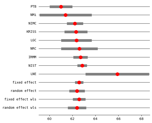
Example Kacker interlaboratory mean
In this example the effect size is the mean of measurements in a lab. We combine the estimates from several labs to estimate and overall average.
[13]:
eff = np.array([61.00, 61.40, 62.21, 62.30, 62.34, 62.60, 62.70, 62.84, 65.90])
var_eff = np.array(
    [0.2025, 1.2100, 0.0900, 0.2025, 0.3844, 0.5625, 0.0676, 0.0225, 1.8225]
)
rownames = ["PTB", "NMi", "NIMC", "KRISS", "LGC", "NRC", "IRMM", "NIST", "LNE"]
[14]:
res2_DL = combine_effects(eff, var_eff, method_re="dl", use_t=True, row_names=rownames)
print("method RE:", res2_DL.method_re)
print(res2_DL.summary_frame())
fig = res2_DL.plot_forest()
fig.set_figheight(6)
fig.set_figwidth(6)
method RE: dl
                         eff    sd_eff     ci_low     ci_upp      w_fe      w_re
PTB                61.000000  0.450000  60.118016  61.881984  0.057436  0.123113
NMi                61.400000  1.100000  59.244040  63.555960  0.009612  0.040314
NIMC               62.210000  0.300000  61.622011  62.797989  0.129230  0.159749
KRISS              62.300000  0.450000  61.418016  63.181984  0.057436  0.123113
LGC                62.340000  0.620000  61.124822  63.555178  0.030257  0.089810
NRC                62.600000  0.750000  61.130027  64.069973  0.020677  0.071005
IRMM               62.700000  0.260000  62.190409  63.209591  0.172052  0.169810
NIST               62.840000  0.150000  62.546005  63.133995  0.516920  0.194471
LNE                65.900000  1.350000  63.254049  68.545951  0.006382  0.028615
fixed effect       62.583397  0.107846  62.334704  62.832090  1.000000       NaN
random effect      62.390139  0.245750  61.823439  62.956838       NaN  1.000000
fixed effect wls   62.583397  0.189889  62.145512  63.021282  1.000000       NaN
random effect wls  62.390139  0.294776  61.710384  63.069893       NaN  1.000000
/opt/hostedtoolcache/Python/3.10.20/x64/lib/python3.10/site-packages/statsmodels/stats/meta_analysis.py:224: InvalidTestWarning: `use_t=True` requires `nobs` for each sample or `ci_func`. Using normal distribution for confidence interval of individual samples.
  ci_low, ci_upp = self.conf_int_samples(alpha=alpha, use_t=use_t)
[15]:
res2_PM = combine_effects(eff, var_eff, method_re="pm", use_t=True, row_names=rownames)
print("method RE:", res2_PM.method_re)
print(res2_PM.summary_frame())
fig = res2_PM.plot_forest()
fig.set_figheight(6)
fig.set_figwidth(6)
method RE: pm
                         eff    sd_eff     ci_low     ci_upp      w_fe      w_re
PTB                61.000000  0.450000  60.118016  61.881984  0.057436  0.125857
NMi                61.400000  1.100000  59.244040  63.555960  0.009612  0.059656
NIMC               62.210000  0.300000  61.622011  62.797989  0.129230  0.143658
KRISS              62.300000  0.450000  61.418016  63.181984  0.057436  0.125857
LGC                62.340000  0.620000  61.124822  63.555178  0.030257  0.104850
NRC                62.600000  0.750000  61.130027  64.069973  0.020677  0.090122
IRMM               62.700000  0.260000  62.190409  63.209591  0.172052  0.147821
NIST               62.840000  0.150000  62.546005  63.133995  0.516920  0.156980
LNE                65.900000  1.350000  63.254049  68.545951  0.006382  0.045201
fixed effect       62.583397  0.107846  62.334704  62.832090  1.000000       NaN
random effect      62.407620  0.338030  61.628120  63.187119       NaN  1.000000
fixed effect wls   62.583397  0.189889  62.145512  63.021282  1.000000       NaN
random effect wls  62.407620  0.338030  61.628120  63.187120       NaN  1.000000
/opt/hostedtoolcache/Python/3.10.20/x64/lib/python3.10/site-packages/statsmodels/stats/meta_analysis.py:224: InvalidTestWarning: `use_t=True` requires `nobs` for each sample or `ci_func`. Using normal distribution for confidence interval of individual samples.
  ci_low, ci_upp = self.conf_int_samples(alpha=alpha, use_t=use_t)

[ ]:
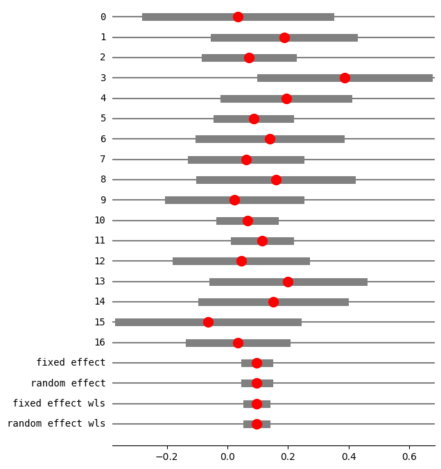
Meta-analysis of proportions
In the following example the random effect variance tau is estimated to be zero. I then change two counts in the data, so the second example has random effects variance greater than zero.
[16]:
import io
[17]:
ss = """\
    study,nei,nci,e1i,c1i,e2i,c2i,e3i,c3i,e4i,c4i
    1,19,22,16.0,20.0,11,12,4.0,8.0,4,3
    2,34,35,22.0,22.0,18,12,15.0,8.0,15,6
    3,72,68,44.0,40.0,21,15,10.0,3.0,3,0
    4,22,20,19.0,12.0,14,5,5.0,4.0,2,3
    5,70,32,62.0,27.0,42,13,26.0,6.0,15,5
    6,183,94,130.0,65.0,80,33,47.0,14.0,30,11
    7,26,50,24.0,30.0,13,18,5.0,10.0,3,9
    8,61,55,51.0,44.0,37,30,19.0,19.0,11,15
    9,36,25,30.0,17.0,23,12,13.0,4.0,10,4
    10,45,35,43.0,35.0,19,14,8.0,4.0,6,0
    11,246,208,169.0,139.0,106,76,67.0,42.0,51,35
    12,386,141,279.0,97.0,170,46,97.0,21.0,73,8
    13,59,32,56.0,30.0,34,17,21.0,9.0,20,7
    14,45,15,42.0,10.0,18,3,9.0,1.0,9,1
    15,14,18,14.0,18.0,13,14,12.0,13.0,9,12
    16,26,19,21.0,15.0,12,10,6.0,4.0,5,1
    17,74,75,,,42,40,,,23,30"""
df3 = pd.read_csv(io.StringIO(ss))
df_12y = df3[["e2i", "nei", "c2i", "nci"]]
# TODO: currently 1 is reference, switch labels
count1, nobs1, count2, nobs2 = df_12y.values.T
dta = df_12y.values.T
[18]:
eff, var_eff = effectsize_2proportions(*dta, statistic="rd")
[19]:
eff, var_eff
[19]:
(array([ 0.03349282,  0.18655462,  0.07107843,  0.38636364,  0.19375   ,
         0.08609464,  0.14      ,  0.06110283,  0.15888889,  0.02222222,
         0.06550969,  0.11417337,  0.04502119,  0.2       ,  0.15079365,
        -0.06477733,  0.03423423]),
 array([0.02409958, 0.01376482, 0.00539777, 0.01989341, 0.01096641,
        0.00376814, 0.01422338, 0.00842011, 0.01639261, 0.01227827,
        0.00211165, 0.00219739, 0.01192067, 0.016     , 0.0143398 ,
        0.02267994, 0.0066352 ]))
[20]:
res5 = combine_effects(
    eff, var_eff, method_re="iterated", use_t=False
)  # , row_names=rownames)
res5_df = res5.summary_frame()
print("method RE:", res5.method_re)
print("RE variance tau2:", res5.tau2)
print(res5.summary_frame())
fig = res5.plot_forest()
fig.set_figheight(8)
fig.set_figwidth(6)
method RE: iterated
RE variance tau2: 0
                        eff    sd_eff    ci_low    ci_upp      w_fe      w_re
0                  0.033493  0.155240 -0.270773  0.337758  0.017454  0.017454
1                  0.186555  0.117324 -0.043395  0.416505  0.030559  0.030559
2                  0.071078  0.073470 -0.072919  0.215076  0.077928  0.077928
3                  0.386364  0.141044  0.109922  0.662805  0.021145  0.021145
4                  0.193750  0.104721 -0.011499  0.398999  0.038357  0.038357
5                  0.086095  0.061385 -0.034218  0.206407  0.111630  0.111630
6                  0.140000  0.119262 -0.093749  0.373749  0.029574  0.029574
7                  0.061103  0.091761 -0.118746  0.240951  0.049956  0.049956
8                  0.158889  0.128034 -0.092052  0.409830  0.025660  0.025660
9                  0.022222  0.110807 -0.194956  0.239401  0.034259  0.034259
10                 0.065510  0.045953 -0.024556  0.155575  0.199199  0.199199
11                 0.114173  0.046876  0.022297  0.206049  0.191426  0.191426
12                 0.045021  0.109182 -0.168971  0.259014  0.035286  0.035286
13                 0.200000  0.126491 -0.047918  0.447918  0.026290  0.026290
14                 0.150794  0.119749 -0.083910  0.385497  0.029334  0.029334
15                -0.064777  0.150599 -0.359945  0.230390  0.018547  0.018547
16                 0.034234  0.081457 -0.125418  0.193887  0.063395  0.063395
fixed effect       0.096212  0.020509  0.056014  0.136410  1.000000       NaN
random effect      0.096212  0.020509  0.056014  0.136410       NaN  1.000000
fixed effect wls   0.096212  0.016521  0.063831  0.128593  1.000000       NaN
random effect wls  0.096212  0.016521  0.063831  0.128593       NaN  1.000000
changing data to have positive random effects variance
[21]:
dta_c = dta.copy()
dta_c.T[0, 0] = 18
dta_c.T[1, 0] = 22
dta_c.T
[21]:
array([[ 18,  19,  12,  22],
       [ 22,  34,  12,  35],
       [ 21,  72,  15,  68],
       [ 14,  22,   5,  20],
       [ 42,  70,  13,  32],
       [ 80, 183,  33,  94],
       [ 13,  26,  18,  50],
       [ 37,  61,  30,  55],
       [ 23,  36,  12,  25],
       [ 19,  45,  14,  35],
       [106, 246,  76, 208],
       [170, 386,  46, 141],
       [ 34,  59,  17,  32],
       [ 18,  45,   3,  15],
       [ 13,  14,  14,  18],
       [ 12,  26,  10,  19],
       [ 42,  74,  40,  75]])
[22]:
eff, var_eff = effectsize_2proportions(*dta_c, statistic="rd")
res5 = combine_effects(
    eff, var_eff, method_re="iterated", use_t=False
)  # , row_names=rownames)
res5_df = res5.summary_frame()
print("method RE:", res5.method_re)
print(res5.summary_frame())
fig = res5.plot_forest()
fig.set_figheight(8)
fig.set_figwidth(6)
method RE: iterated
                        eff    sd_eff    ci_low    ci_upp      w_fe      w_re
0                  0.401914  0.117873  0.170887  0.632940  0.029850  0.038415
1                  0.304202  0.114692  0.079410  0.528993  0.031529  0.040258
2                  0.071078  0.073470 -0.072919  0.215076  0.076834  0.081017
3                  0.386364  0.141044  0.109922  0.662805  0.020848  0.028013
4                  0.193750  0.104721 -0.011499  0.398999  0.037818  0.046915
5                  0.086095  0.061385 -0.034218  0.206407  0.110063  0.102907
6                  0.140000  0.119262 -0.093749  0.373749  0.029159  0.037647
7                  0.061103  0.091761 -0.118746  0.240951  0.049255  0.058097
8                  0.158889  0.128034 -0.092052  0.409830  0.025300  0.033270
9                  0.022222  0.110807 -0.194956  0.239401  0.033778  0.042683
10                 0.065510  0.045953 -0.024556  0.155575  0.196403  0.141871
11                 0.114173  0.046876  0.022297  0.206049  0.188739  0.139144
12                 0.045021  0.109182 -0.168971  0.259014  0.034791  0.043759
13                 0.200000  0.126491 -0.047918  0.447918  0.025921  0.033985
14                 0.150794  0.119749 -0.083910  0.385497  0.028922  0.037383
15                -0.064777  0.150599 -0.359945  0.230390  0.018286  0.024884
16                 0.034234  0.081457 -0.125418  0.193887  0.062505  0.069751
fixed effect       0.110252  0.020365  0.070337  0.150167  1.000000       NaN
random effect      0.117633  0.024913  0.068804  0.166463       NaN  1.000000
fixed effect wls   0.110252  0.022289  0.066567  0.153937  1.000000       NaN
random effect wls  0.117633  0.024913  0.068804  0.166463       NaN  1.000000

[23]:
res5 = combine_effects(eff, var_eff, method_re="chi2", use_t=False)
res5_df = res5.summary_frame()
print("method RE:", res5.method_re)
print(res5.summary_frame())
fig = res5.plot_forest()
fig.set_figheight(8)
fig.set_figwidth(6)
method RE: chi2
                        eff    sd_eff    ci_low    ci_upp      w_fe      w_re
0                  0.401914  0.117873  0.170887  0.632940  0.029850  0.036114
1                  0.304202  0.114692  0.079410  0.528993  0.031529  0.037940
2                  0.071078  0.073470 -0.072919  0.215076  0.076834  0.080779
3                  0.386364  0.141044  0.109922  0.662805  0.020848  0.025973
4                  0.193750  0.104721 -0.011499  0.398999  0.037818  0.044614
5                  0.086095  0.061385 -0.034218  0.206407  0.110063  0.105901
6                  0.140000  0.119262 -0.093749  0.373749  0.029159  0.035356
7                  0.061103  0.091761 -0.118746  0.240951  0.049255  0.056098
8                  0.158889  0.128034 -0.092052  0.409830  0.025300  0.031063
9                  0.022222  0.110807 -0.194956  0.239401  0.033778  0.040357
10                 0.065510  0.045953 -0.024556  0.155575  0.196403  0.154854
11                 0.114173  0.046876  0.022297  0.206049  0.188739  0.151236
12                 0.045021  0.109182 -0.168971  0.259014  0.034791  0.041435
13                 0.200000  0.126491 -0.047918  0.447918  0.025921  0.031761
14                 0.150794  0.119749 -0.083910  0.385497  0.028922  0.035095
15                -0.064777  0.150599 -0.359945  0.230390  0.018286  0.022976
16                 0.034234  0.081457 -0.125418  0.193887  0.062505  0.068449
fixed effect       0.110252  0.020365  0.070337  0.150167  1.000000       NaN
random effect      0.115580  0.023557  0.069410  0.161751       NaN  1.000000
fixed effect wls   0.110252  0.022289  0.066567  0.153937  1.000000       NaN
random effect wls  0.115580  0.024241  0.068068  0.163093       NaN  1.000000

Replicate fixed effect analysis using GLM with var_weights
combine_effects computes weighted average estimates which can be replicated using GLM with var_weights or with WLS. The scale option in GLM.fit can be used to replicate fixed meta-analysis with fixed and with HKSJ/WLS scale
[24]:
from statsmodels.genmod.generalized_linear_model import GLM
[25]:
eff, var_eff = effectsize_2proportions(*dta_c, statistic="or")
res = combine_effects(eff, var_eff, method_re="chi2", use_t=False)
res_frame = res.summary_frame()
print(res_frame.iloc[-4:])
                        eff    sd_eff    ci_low    ci_upp  w_fe  w_re
fixed effect       0.428037  0.090287  0.251076  0.604997   1.0   NaN
random effect      0.429520  0.091377  0.250425  0.608615   NaN   1.0
fixed effect wls   0.428037  0.090798  0.250076  0.605997   1.0   NaN
random effect wls  0.429520  0.091595  0.249997  0.609044   NaN   1.0
We need to fix scale=1 in order to replicate standard errors for the usual meta-analysis.
[26]:
weights = 1 / var_eff
mod_glm = GLM(eff, np.ones(len(eff)), var_weights=weights)
res_glm = mod_glm.fit(scale=1.0)
print(res_glm.summary().tables[1])
==============================================================================
                 coef    std err          z      P>|z|      [0.025      0.975]
------------------------------------------------------------------------------
const          0.4280      0.090      4.741      0.000       0.251       0.605
==============================================================================
[27]:
# check results
res_glm.scale, res_glm.conf_int() - res_frame.loc[
    "fixed effect", ["ci_low", "ci_upp"]
].values
[27]:
(array(1.), array([[-5.55111512e-17, 0.00000000e+00]]))
Using HKSJ variance adjustment in meta-analysis is equivalent to estimating the scale using pearson chi2, which is also the default for the gaussian family.
[28]:
res_glm = mod_glm.fit(scale="x2")
print(res_glm.summary().tables[1])
==============================================================================
                 coef    std err          z      P>|z|      [0.025      0.975]
------------------------------------------------------------------------------
const          0.4280      0.091      4.714      0.000       0.250       0.606
==============================================================================
[29]:
# check results
res_glm.scale, res_glm.conf_int() - res_frame.loc[
    "fixed effect", ["ci_low", "ci_upp"]
].values
[29]:
(np.float64(1.0113358914264383), array([[-0.00100017, 0.00100017]]))
Mantel-Hanszel odds-ratio using contingency tables
The fixed effect for the log-odds-ratio using the Mantel-Hanszel can be directly computed using StratifiedTable.
We need to create a 2 x 2 x k contingency table to be used with StratifiedTable.
[30]:
t, nt, c, nc = dta_c
counts = np.column_stack([t, nt - t, c, nc - c])
ctables = counts.T.reshape(2, 2, -1)
ctables[:, :, 0]
[30]:
array([[18,  1],
       [12, 10]])
[31]:
counts[0]
[31]:
array([18, 1, 12, 10])
[32]:
dta_c.T[0]
[32]:
array([18, 19, 12, 22])
[33]:
import statsmodels.stats.api as smstats
[34]:
st = smstats.StratifiedTable(ctables.astype(np.float64))
compare pooled log-odds-ratio and standard error to R meta package
[35]:
st.logodds_pooled, st.logodds_pooled - 0.4428186730553189 # R meta
[35]:
(np.float64(0.4428186730553187), np.float64(-2.220446049250313e-16))
[36]:
st.logodds_pooled_se, st.logodds_pooled_se - 0.08928560091027186 # R meta
[36]:
(np.float64(0.08928560091027186), np.float64(0.0))
[37]:
st.logodds_pooled_confint()
[37]:
(np.float64(0.2678221109331691), np.float64(0.6178152351774683))
[38]:
print(st.test_equal_odds())
pvalue      0.34496419319878724
statistic   17.64707987033203
[39]:
print(st.test_null_odds())
pvalue      6.615053645964153e-07
statistic   24.724136624311814
check conversion to stratified contingency table
Row sums of each table are the sample sizes for treatment and control experiments
[40]:
ctables.sum(1)
[40]:
array([[ 19,  34,  72,  22,  70, 183,  26,  61,  36,  45, 246, 386,  59,
         45,  14,  26,  74],
       [ 22,  35,  68,  20,  32,  94,  50,  55,  25,  35, 208, 141,  32,
         15,  18,  19,  75]])
[41]:
nt, nc
[41]:
(array([ 19,  34,  72,  22,  70, 183,  26,  61,  36,  45, 246, 386,  59,
         45,  14,  26,  74]),
 array([ 22,  35,  68,  20,  32,  94,  50,  55,  25,  35, 208, 141,  32,
         15,  18,  19,  75]))
Results from R meta package
> res_mb_hk = metabin(e2i, nei, c2i, nci, data=dat2, sm="OR", Q.Cochrane=FALSE, method="MH", method.tau="DL", hakn=FALSE, backtransf=FALSE)
> res_mb_hk
     logOR            95%-CI %W(fixed) %W(random)
1   2.7081 [ 0.5265; 4.8896]       0.3        0.7
2   1.2567 [ 0.2658; 2.2476]       2.1        3.2
3   0.3749 [-0.3911; 1.1410]       5.4        5.4
4   1.6582 [ 0.3245; 2.9920]       0.9        1.8
5   0.7850 [-0.0673; 1.6372]       3.5        4.4
6   0.3617 [-0.1528; 0.8762]      12.1       11.8
7   0.5754 [-0.3861; 1.5368]       3.0        3.4
8   0.2505 [-0.4881; 0.9892]       6.1        5.8
9   0.6506 [-0.3877; 1.6889]       2.5        3.0
10  0.0918 [-0.8067; 0.9903]       4.5        3.9
11  0.2739 [-0.1047; 0.6525]      23.1       21.4
12  0.4858 [ 0.0804; 0.8911]      18.6       18.8
13  0.1823 [-0.6830; 1.0476]       4.6        4.2
14  0.9808 [-0.4178; 2.3795]       1.3        1.6
15  1.3122 [-1.0055; 3.6299]       0.4        0.6
16 -0.2595 [-1.4450; 0.9260]       3.1        2.3
17  0.1384 [-0.5076; 0.7844]       8.5        7.6

Number of studies combined: k = 17

                      logOR           95%-CI    z  p-value
Fixed effect model   0.4428 [0.2678; 0.6178] 4.96 < 0.0001
Random effects model 0.4295 [0.2504; 0.6086] 4.70 < 0.0001

Quantifying heterogeneity:
 tau^2 = 0.0017 [0.0000; 0.4589]; tau = 0.0410 [0.0000; 0.6774];
 I^2 = 1.1% [0.0%; 51.6%]; H = 1.01 [1.00; 1.44]

Test of heterogeneity:
     Q d.f. p-value
 16.18   16  0.4404

Details on meta-analytical method:
- Mantel-Haenszel method
- DerSimonian-Laird estimator for tau^2
- Jackson method for confidence interval of tau^2 and tau

> res_mb_hk$TE.fixed
[1] 0.4428186730553189
> res_mb_hk$seTE.fixed
[1] 0.08928560091027186
> c(res_mb_hk$lower.fixed, res_mb_hk$upper.fixed)
[1] 0.2678221109331694 0.6178152351774684
[42]:
print(st.summary())
                   Estimate   LCB    UCB
-----------------------------------------
Pooled odds           1.557   1.307 1.855
Pooled log odds       0.443   0.268 0.618
Pooled risk ratio     1.270

                 Statistic P-value
-----------------------------------
Test of OR=1        24.724   0.000
Test constant OR    17.647   0.345

-----------------------
Number of tables   17
Min n              32
Max n             527
Avg n             139
Total n          2362
-----------------------