Prediction (out of sample)
[1]:
%matplotlib inline
[2]:
import numpy as np
import matplotlib.pyplot as plt

import statsmodels.api as sm

plt.rc("figure", figsize=(16, 8))
plt.rc("font", size=14)
Artificial data
[3]:
nsample = 50
sig = 0.25
x1 = np.linspace(0, 20, nsample)
X = np.column_stack((x1, np.sin(x1), (x1 - 5) ** 2))
X = sm.add_constant(X)
beta = [5.0, 0.5, 0.5, -0.02]
y_true = np.dot(X, beta)
y = y_true + sig * np.random.normal(size=nsample)
Estimation
[4]:
olsmod = sm.OLS(y, X)
olsres = olsmod.fit()
print(olsres.summary())
                            OLS Regression Results
==============================================================================
Dep. Variable:                      y   R-squared:                       0.985
Model:                            OLS   Adj. R-squared:                  0.984
Method:                 Least Squares   F-statistic:                     1013.
Date:                Fri, 12 Jun 2026   Prob (F-statistic):           5.30e-42
Time:                        12:50:42   Log-Likelihood:                 4.6393
No. Observations:                  50   AIC:                            -1.279
Df Residuals:                      46   BIC:                             6.369
Df Model:                           3
Covariance Type:            nonrobust
==============================================================================
                 coef    std err          t      P>|t|      [0.025      0.975]
------------------------------------------------------------------------------
const          5.1203      0.078     65.338      0.000       4.963       5.278
x1             0.4883      0.012     40.403      0.000       0.464       0.513
x2             0.4821      0.048     10.147      0.000       0.386       0.578
x3            -0.0197      0.001    -18.571      0.000      -0.022      -0.018
==============================================================================
Omnibus:                        1.226   Durbin-Watson:                   2.475
Prob(Omnibus):                  0.542   Jarque-Bera (JB):                1.096
Skew:                          -0.350   Prob(JB):                        0.578
Kurtosis:                       2.809   Cond. No.                         221.
==============================================================================

Notes:
[1] Standard Errors assume that the covariance matrix of the errors is correctly specified.
In-sample prediction
[5]:
ypred = olsres.predict(X)
print(ypred)
[ 4.62760815  5.09542147  5.52522984  5.89075973  6.17521962  6.37405873
  6.49571477  6.56022757  6.59594667  6.6348735   6.70740369  6.83733314
  7.03794839  7.30984373  7.64082351  8.00790589  8.38109867  8.72832693
  9.02070284  9.23727188  9.36845555  9.41762515  9.40054786  9.34279622
  9.27554667  9.23045731  9.23446661  9.30536744  9.44888381  9.65773038
  9.91280946 10.18634867 10.44646391 10.66239778 10.80957296 10.8736302
 10.85278746 10.75813278 10.61180243 10.44334411 10.28486223 10.16574334
 10.10782793 10.12182216 10.20553882 10.34425671 10.51313928 10.68131523
 10.81695051 10.89247867]
Create a new sample of explanatory variables Xnew, predict and plot
[6]:
x1n = np.linspace(20.5, 25, 10)
Xnew = np.column_stack((x1n, np.sin(x1n), (x1n - 5) ** 2))
Xnew = sm.add_constant(Xnew)
ynewpred = olsres.predict(Xnew)  # predict out of sample
print(ynewpred)
[10.87654414 10.7330979  10.48104572 10.16347146  9.83708861  9.5583549
  9.36964942  9.28889681  9.30517861  9.38140652]
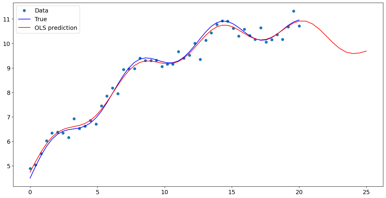
Plot comparison
[7]:
import matplotlib.pyplot as plt

fig, ax = plt.subplots()
ax.plot(x1, y, "o", label="Data")
ax.plot(x1, y_true, "b-", label="True")
ax.plot(np.hstack((x1, x1n)), np.hstack((ypred, ynewpred)), "r", label="OLS prediction")
ax.legend(loc="best")
[7]:
<matplotlib.legend.Legend at 0x7f118a075570>
Predicting with Formulas
Using formulas can make both estimation and prediction a lot easier
[8]:
from statsmodels.formula.api import ols

data = {"x1": x1, "y": y}

res = ols("y ~ x1 + np.sin(x1) + I((x1-5)**2)", data=data).fit()
We use the I to indicate use of the Identity transform. Ie., we do not want any expansion magic from using **2
[9]:
res.params
[9]:
Intercept           5.120274
x1                  0.488304
np.sin(x1)          0.482090
I((x1 - 5) ** 2)   -0.019707
dtype: float64
Now we only have to pass the single variable and we get the transformed right-hand side variables automatically
[10]:
res.predict(exog=dict(x1=x1n))
[10]:
0    10.876544
1    10.733098
2    10.481046
3    10.163471
4     9.837089
5     9.558355
6     9.369649
7     9.288897
8     9.305179
9     9.381407
dtype: float64