The Theta Model
The Theta model of Assimakopoulos & Nikolopoulos (2000) is a simple method for forecasting the involves fitting two \(\theta\)-lines, forecasting the lines using a Simple Exponential Smoother, and then combining the forecasts from the two lines to produce the final forecast. The model is implemented in steps:
Test for seasonality
Deseasonalize if seasonality is detected
Estimate \(\alpha\) by fitting an SES model to the data and \(b_0\) by OLS.
Forecast the series
Reseasonalize if the data was deseasonalized.
The seasonality test examines the ACF at the seasonal lag \(m\). If this lag is significantly different from zero, then the data is deseasonalized using statsmodels.tsa.seasonal_decompose using either a multiplicative method (default) or additive.
The parameters of the model are \(b_0\) and \(\alpha\) where \(b_0\) is estimated from the OLS regression
and \(\alpha\) is the SES smoothing parameter in
The forecasts are then
Ultimately \(\theta\) only plays a role in determining how much the trend is damped. If \(\theta\) is very large, then the forecast of the model is identical to that from an Integrated Moving Average with a drift,
Finally, the forecasts are reseasonalized if needed.
This module is based on:
Assimakopoulos, V., & Nikolopoulos, K. (2000). The theta model: a decomposition approach to forecasting. International journal of forecasting, 16(4), 521-530.
Hyndman, R. J., & Billah, B. (2003). Unmasking the Theta method. International Journal of Forecasting, 19(2), 287-290.
Fioruci, J. A., Pellegrini, T. R., Louzada, F., & Petropoulos, F. (2015). The optimized theta method. arXiv preprint arXiv:1503.03529.
Imports
We start with the standard set of imports and some tweaks to the default matplotlib style.
[1]:
import matplotlib.pyplot as plt
import numpy as np
import pandas as pd
import pandas_datareader as pdr
import seaborn as sns

plt.rc("figure", figsize=(16, 8))
plt.rc("font", size=15)
plt.rc("lines", linewidth=3)
sns.set_style("darkgrid")
Load some Data
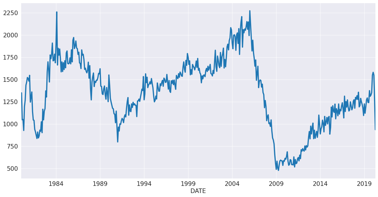
We will first look at housing starts using US data. This series is clearly seasonal but does not have a clear trend during the same.
[2]:
reader = pdr.fred.FredReader(["HOUST"], start="1980-01-01", end="2020-04-01")
data = reader.read()
housing = data.HOUST
housing.index.freq = housing.index.inferred_freq
ax = housing.plot()
We specify the model without any options and fit it. The summary shows that the data was deseasonalized using the multiplicative method. The drift is modest and negative, and the smoothing parameter is fairly low.
[3]:
from statsmodels.tsa.forecasting.theta import ThetaModel

tm = ThetaModel(housing)
res = tm.fit()
print(res.summary())
                              ThetaModel Results
==============================================================================
Dep. Variable:                  HOUST   No. Observations:                  484
Method:                       OLS/SES   Deseasonalized:                   True
Date:                Sun, 14 Jun 2026   Deseas. Method:         Multiplicative
Time:                        23:03:25   Period:                             12
Sample:                    01-01-1980
                         - 04-01-2020
   Parameter Estimates
=========================
           Parameters
-------------------------
b0    -0.9185839033748175
alpha  0.6165175851279336
-------------------------
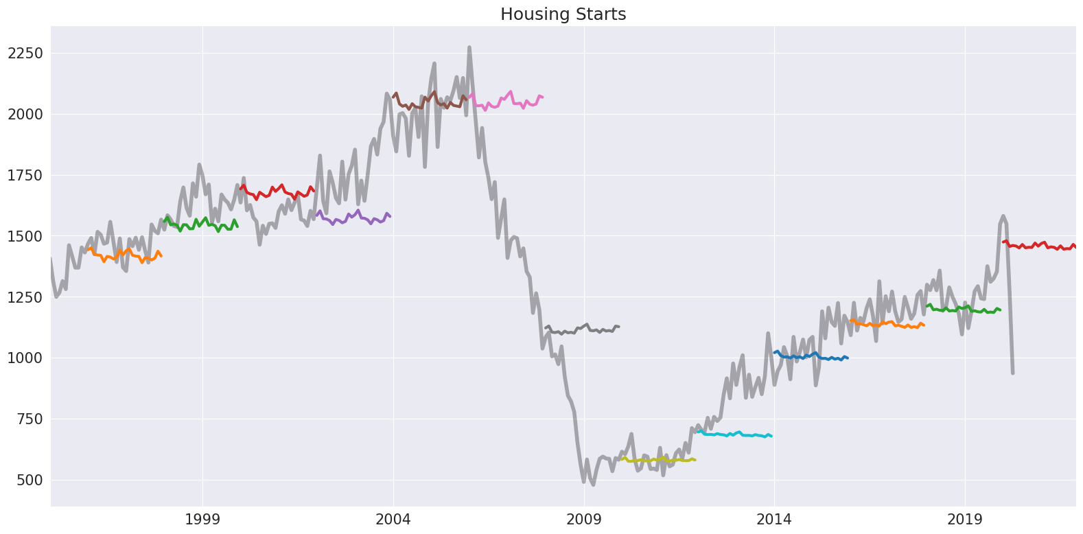
The model is first and foremost a forecasting method. Forecasts are produced using the forecast method from the fitted model. Below, we produce a hedgehog plot by forecasting 2-years ahead every 2 years.
Note: the default \(\theta\) is 2.
[4]:
forecasts = {"housing": housing}
for year in range(1995, 2020, 2):
    sub = housing[: str(year)]
    res = ThetaModel(sub).fit()
    fcast = res.forecast(24)
    forecasts[str(year)] = fcast
forecasts = pd.DataFrame(forecasts)
ax = forecasts["1995":].plot(legend=False)
children = ax.get_children()
children[0].set_linewidth(4)
children[0].set_alpha(0.3)
children[0].set_color("#000000")
ax.set_title("Housing Starts")
plt.tight_layout(pad=1.0)
We could alternatively fit the log of the data. Here it makes more sense to force the deseasonalizing to use the additive method, if needed. We also fit the model parameters using MLE. This method fits the IMA
where \(\hat{\alpha}\) = \(\min(\hat{\gamma}+1, 0.9998)\) using statsmodels.tsa.SARIMAX. The parameters are similar although the drift is closer to zero.
[5]:
tm = ThetaModel(np.log(housing), method="additive")
res = tm.fit(use_mle=True)
print(res.summary())
                              ThetaModel Results
==============================================================================
Dep. Variable:                  HOUST   No. Observations:                  484
Method:                           MLE   Deseasonalized:                   True
Date:                Sun, 14 Jun 2026   Deseas. Method:               Additive
Time:                        23:03:28   Period:                             12
Sample:                    01-01-1980
                         - 04-01-2020
    Parameter Estimates
============================
            Parameters
----------------------------
b0    -0.0004318336863785846
alpha     0.6699525580249173
----------------------------
The forecast only depends on the forecast trend component,
the forecast from the SES (which does not change with the horizon), and the seasonal. These three components are available using the forecast_components. This allows forecasts to be constructed using multiple choices of \(\theta\) using the weight expression above.
[6]:
res.forecast_components(12)
[6]:
| trend | ses | seasonal | |
|---|---|---|---|
| 2020-05-01 | -0.000645 | 6.964198 | -0.001244 |
| 2020-06-01 | -0.001076 | 6.964198 | -0.006883 |
| 2020-07-01 | -0.001508 | 6.964198 | 0.002998 |
| 2020-08-01 | -0.001940 | 6.964198 | -0.003822 |
| 2020-09-01 | -0.002372 | 6.964198 | -0.003926 |
| 2020-10-01 | -0.002804 | 6.964198 | -0.004022 |
| 2020-11-01 | -0.003236 | 6.964198 | 0.008544 |
| 2020-12-01 | -0.003667 | 6.964198 | -0.000706 |
| 2021-01-01 | -0.004099 | 6.964198 | 0.005247 |
| 2021-02-01 | -0.004531 | 6.964198 | 0.009951 |
| 2021-03-01 | -0.004963 | 6.964198 | -0.004527 |
| 2021-04-01 | -0.005395 | 6.964198 | -0.001611 |
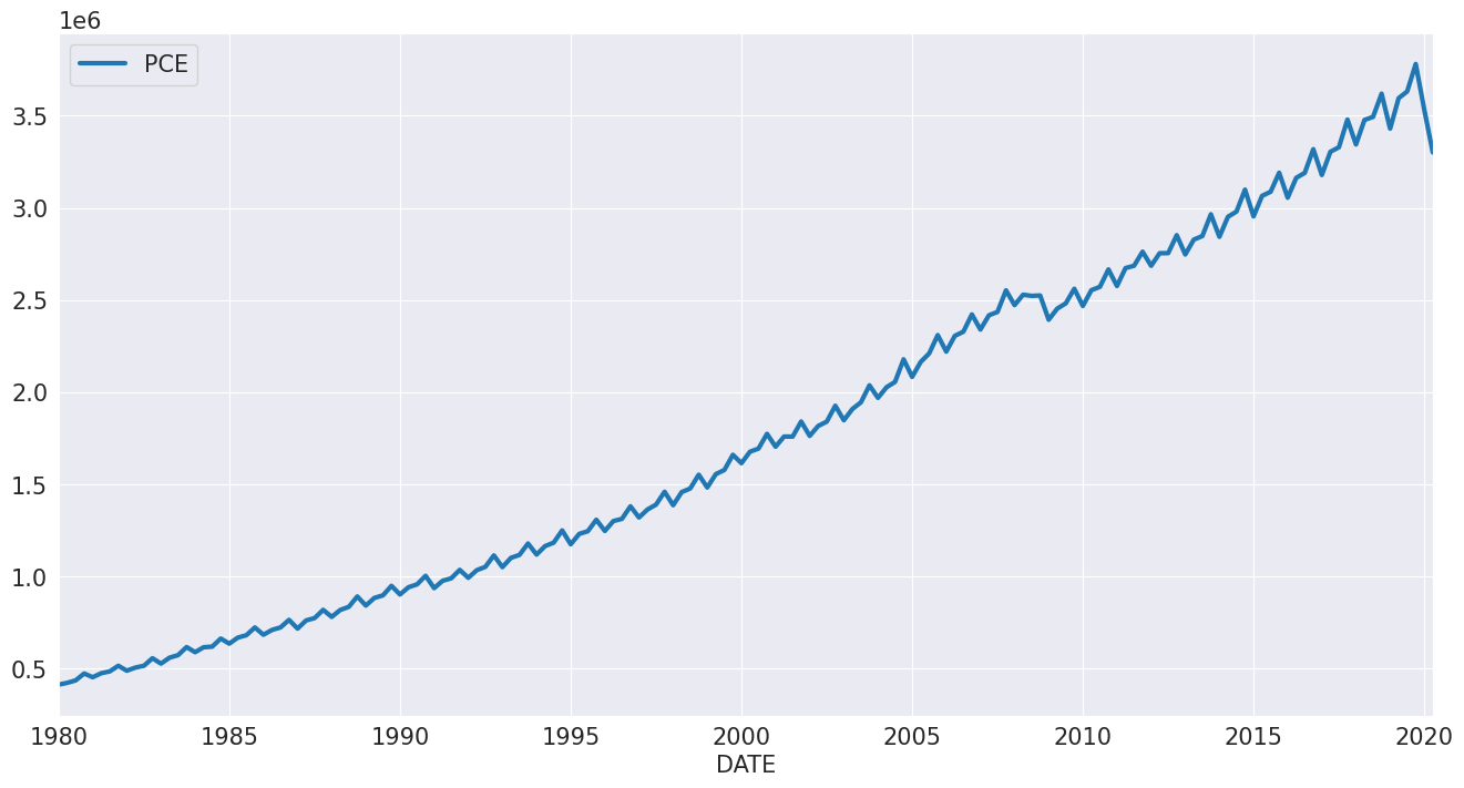
Personal Consumption Expenditure
We next look at personal consumption expenditure. This series has a clear seasonal component and a drift.
[7]:
reader = pdr.fred.FredReader(["NA000349Q"], start="1980-01-01", end="2020-04-01")
pce = reader.read()
pce.columns = ["PCE"]
pce.index.freq = "QS-OCT"
_ = pce.plot()
Since this series is always positive, we model the \(\ln\).
[8]:
mod = ThetaModel(np.log(pce))
res = mod.fit()
print(res.summary())
                              ThetaModel Results
==============================================================================
Dep. Variable:                    PCE   No. Observations:                  162
Method:                       OLS/SES   Deseasonalized:                   True
Date:                Sun, 14 Jun 2026   Deseas. Method:         Multiplicative
Time:                        23:03:35   Period:                              4
Sample:                    01-01-1980
                         - 04-01-2020
   Parameter Estimates
=========================
           Parameters
-------------------------
b0    0.01303597716708746
alpha  0.9998852087678992
-------------------------
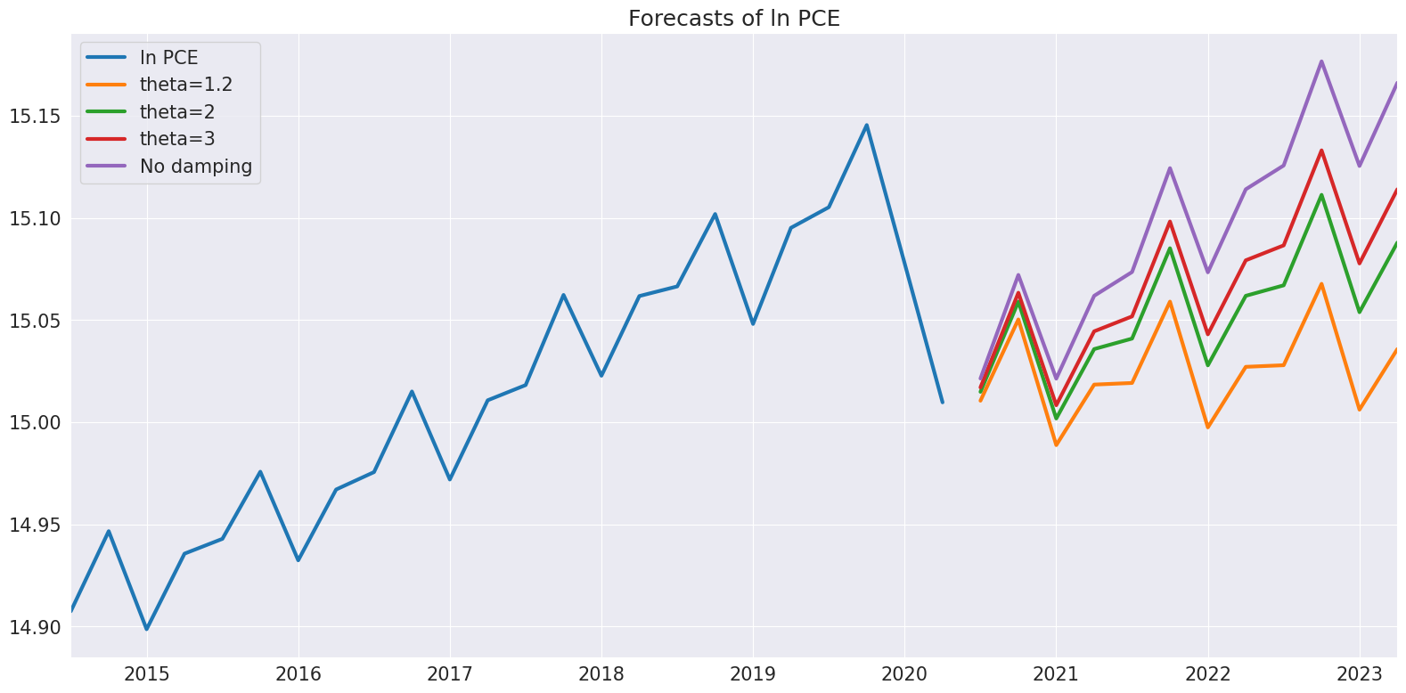
Next we explore differences in the forecast as \(\theta\) changes. When \(\theta\) is close to 1, the drift is nearly absent. As \(\theta\) increases, the drift becomes more obvious.
[9]:
forecasts = pd.DataFrame(
    {
        "ln PCE": np.log(pce.PCE),
        "theta=1.2": res.forecast(12, theta=1.2),
        "theta=2": res.forecast(12),
        "theta=3": res.forecast(12, theta=3),
        "No damping": res.forecast(12, theta=np.inf),
    }
)
_ = forecasts.tail(36).plot()
plt.title("Forecasts of ln PCE")
plt.tight_layout(pad=1.0)
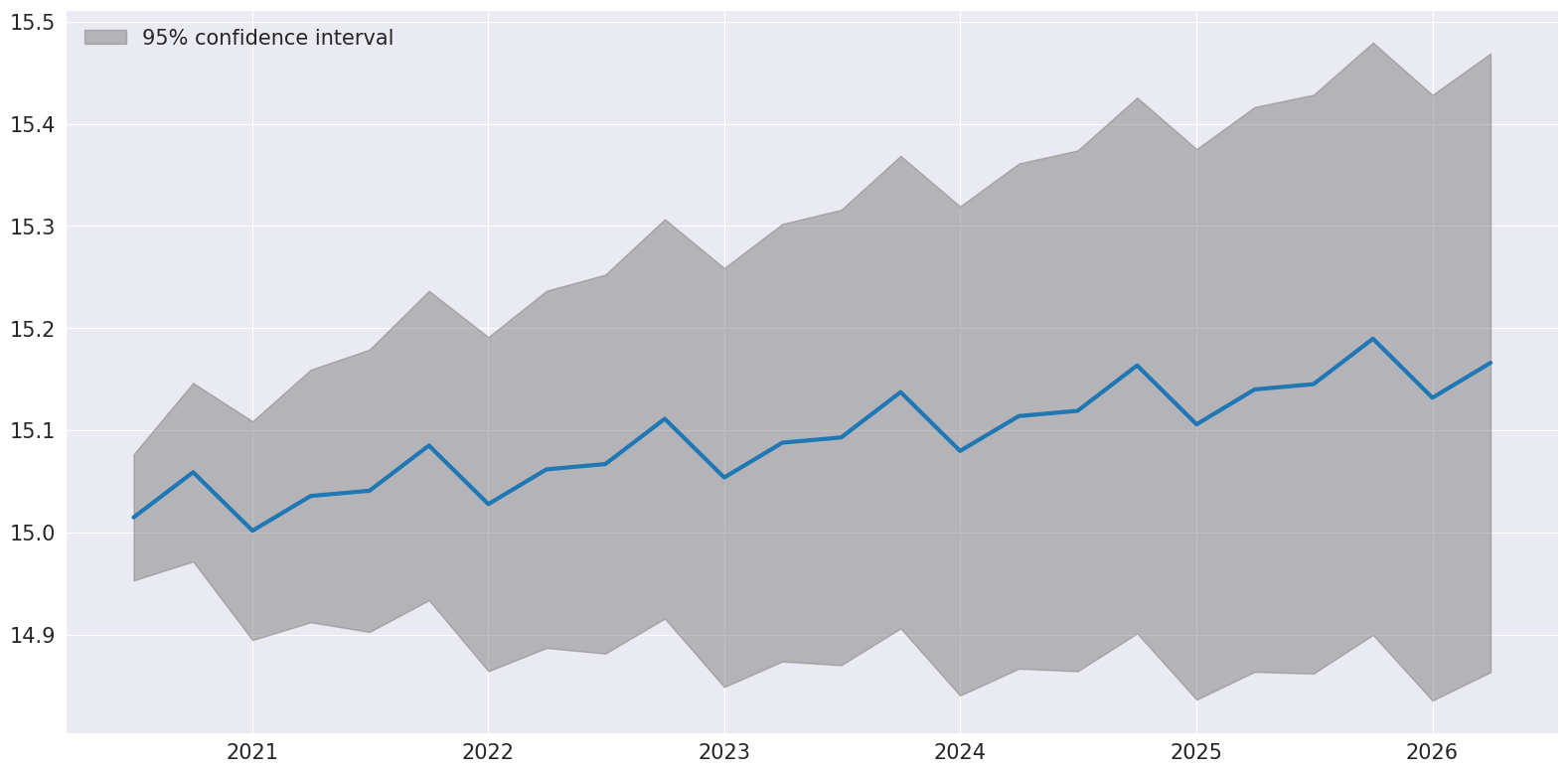
Finally, plot_predict can be used to visualize the predictions and prediction intervals which are constructed assuming the IMA is true.
[10]:
ax = res.plot_predict(24, theta=2)
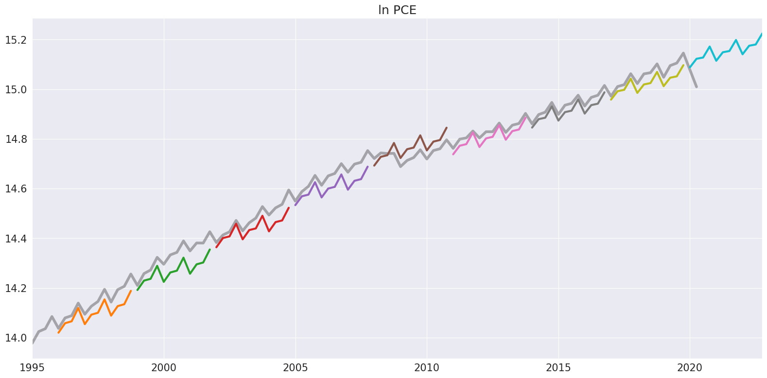
We conclude by producing a hedgehog plot using 2-year non-overlapping samples.
[11]:
ln_pce = np.log(pce.PCE)
forecasts = {"ln PCE": ln_pce}
for year in range(1995, 2020, 3):
    sub = ln_pce[: str(year)]
    res = ThetaModel(sub).fit()
    fcast = res.forecast(12)
    forecasts[str(year)] = fcast
forecasts = pd.DataFrame(forecasts)
ax = forecasts["1995":].plot(legend=False)
children = ax.get_children()
children[0].set_linewidth(4)
children[0].set_alpha(0.3)
children[0].set_color("#000000")
ax.set_title("ln PCE")
plt.tight_layout(pad=1.0)