Robust Linear Models
[1]:
%matplotlib inline
[2]:
import numpy as np
import statsmodels.api as sm
import matplotlib.pyplot as plt
from statsmodels.sandbox.regression.predstd import wls_prediction_std
Estimation
Load data:
[3]:
data = sm.datasets.stackloss.load(as_pandas=False)
data.exog = sm.add_constant(data.exog)
Huber’s T norm with the (default) median absolute deviation scaling
[4]:
huber_t = sm.RLM(data.endog, data.exog, M=sm.robust.norms.HuberT())
hub_results = huber_t.fit()
print(hub_results.params)
print(hub_results.bse)
print(hub_results.summary(yname='y',
            xname=['var_%d' % i for i in range(len(hub_results.params))]))
[-41.02649835   0.82938433   0.92606597  -0.12784672]
[9.79189854 0.11100521 0.30293016 0.12864961]
                    Robust linear Model Regression Results
==============================================================================
Dep. Variable:                      y   No. Observations:                   21
Model:                            RLM   Df Residuals:                       17
Method:                          IRLS   Df Model:                            3
Norm:                          HuberT
Scale Est.:                       mad
Cov Type:                          H1
Date:                Tue, 02 Feb 2021
Time:                        06:52:45
No. Iterations:                    19
==============================================================================
                 coef    std err          z      P>|z|      [0.025      0.975]
------------------------------------------------------------------------------
var_0        -41.0265      9.792     -4.190      0.000     -60.218     -21.835
var_1          0.8294      0.111      7.472      0.000       0.612       1.047
var_2          0.9261      0.303      3.057      0.002       0.332       1.520
var_3         -0.1278      0.129     -0.994      0.320      -0.380       0.124
==============================================================================

If the model instance has been used for another fit with different fit parameters, then the fit options might not be the correct ones anymore .
Huber’s T norm with ‘H2’ covariance matrix
[5]:
hub_results2 = huber_t.fit(cov="H2")
print(hub_results2.params)
print(hub_results2.bse)
[-41.02649835   0.82938433   0.92606597  -0.12784672]
[9.08950419 0.11945975 0.32235497 0.11796313]
Andrew’s Wave norm with Huber’s Proposal 2 scaling and ‘H3’ covariance matrix
[6]:
andrew_mod = sm.RLM(data.endog, data.exog, M=sm.robust.norms.AndrewWave())
andrew_results = andrew_mod.fit(scale_est=sm.robust.scale.HuberScale(), cov="H3")
print('Parameters: ', andrew_results.params)
Parameters: [-40.8817957 0.79276138 1.04857556 -0.13360865]
See help(sm.RLM.fit) for more options and module sm.robust.scale for scale options
Comparing OLS and RLM
Artificial data with outliers:
[7]:
nsample = 50
x1 = np.linspace(0, 20, nsample)
X = np.column_stack((x1, (x1-5)**2))
X = sm.add_constant(X)
sig = 0.3   # smaller error variance makes OLS<->RLM contrast bigger
beta = [5, 0.5, -0.0]
y_true2 = np.dot(X, beta)
y2 = y_true2 + sig*1. * np.random.normal(size=nsample)
y2[[39,41,43,45,48]] -= 5   # add some outliers (10% of nsample)
Example 1: quadratic function with linear truth
Note that the quadratic term in OLS regression will capture outlier effects.
[8]:
res = sm.OLS(y2, X).fit()
print(res.params)
print(res.bse)
print(res.predict())
[ 4.9399875   0.54301113 -0.01461384]
[0.44996437 0.06946843 0.00614688]
[ 4.57464158  4.85349246  5.12747409  5.39658648  5.66082961  5.92020349
  6.17470812  6.4243435   6.66910964  6.90900652  7.14403415  7.37419253
  7.59948167  7.81990155  8.03545218  8.24613356  8.45194569  8.65288857
  8.84896221  9.04016659  9.22650172  9.4079676   9.58456423  9.75629162
  9.92314975 10.08513863 10.24225826 10.39450864 10.54188977 10.68440166
 10.82204429 10.95481767 11.0827218  11.20575668 11.32392231 11.4372187
 11.54564583 11.64920371 11.74789234 11.84171172 11.93066185 12.01474273
 12.09395437 12.16829675 12.23776988 12.30237376 12.36210839 12.41697377
 12.4669699  12.51209678]
Estimate RLM:
[9]:
resrlm = sm.RLM(y2, X).fit()
print(resrlm.params)
print(resrlm.bse)
[ 4.84780243e+00  5.33332553e-01 -4.59650485e-03]
[0.15278692 0.02358824 0.00208719]
Draw a plot to compare OLS estimates to the robust estimates:
[10]:
fig = plt.figure(figsize=(12,8))
ax = fig.add_subplot(111)
ax.plot(x1, y2, 'o',label="data")
ax.plot(x1, y_true2, 'b-', label="True")
prstd, iv_l, iv_u = wls_prediction_std(res)
ax.plot(x1, res.fittedvalues, 'r-', label="OLS")
ax.plot(x1, iv_u, 'r--')
ax.plot(x1, iv_l, 'r--')
ax.plot(x1, resrlm.fittedvalues, 'g.-', label="RLM")
ax.legend(loc="best")
[10]:
<matplotlib.legend.Legend at 0x7f35cd59ced0>
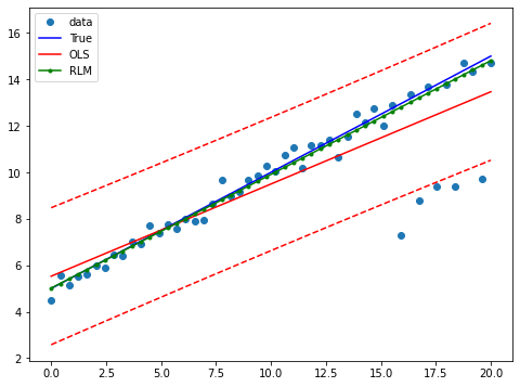
Example 2: linear function with linear truth
Fit a new OLS model using only the linear term and the constant:
[11]:
X2 = X[:,[0,1]]
res2 = sm.OLS(y2, X2).fit()
print(res2.params)
print(res2.bse)
[5.52901458 0.39687276]
[0.3933935  0.03389637]
Estimate RLM:
[12]:
resrlm2 = sm.RLM(y2, X2).fit()
print(resrlm2.params)
print(resrlm2.bse)
[5.01652461 0.48945402]
[0.12230441 0.01053824]
Draw a plot to compare OLS estimates to the robust estimates:
[13]:
prstd, iv_l, iv_u = wls_prediction_std(res2)

fig, ax = plt.subplots(figsize=(8,6))
ax.plot(x1, y2, 'o', label="data")
ax.plot(x1, y_true2, 'b-', label="True")
ax.plot(x1, res2.fittedvalues, 'r-', label="OLS")
ax.plot(x1, iv_u, 'r--')
ax.plot(x1, iv_l, 'r--')
ax.plot(x1, resrlm2.fittedvalues, 'g.-', label="RLM")
legend = ax.legend(loc="best")