VARMAX models
This is a brief introduction notebook to VARMAX models in statsmodels. The VARMAX model is generically specified as:
where \(y_t\) is a \(\text{k_endog} \times 1\) vector.
[1]:
%matplotlib inline
[2]:
import numpy as np
import pandas as pd
import statsmodels.api as sm
import matplotlib.pyplot as plt
[3]:
dta = sm.datasets.webuse('lutkepohl2', 'https://www.stata-press.com/data/r12/')
dta.index = dta.qtr
dta.index.freq = dta.index.inferred_freq
endog = dta.loc['1960-04-01':'1978-10-01', ['dln_inv', 'dln_inc', 'dln_consump']]
Model specification
The VARMAX class in statsmodels allows estimation of VAR, VMA, and VARMA models (through the order argument), optionally with a constant term (via the trend argument). Exogenous regressors may also be included (as usual in statsmodels, by the exog argument), and in this way a time trend may be added. Finally, the class allows measurement error (via the measurement_error argument) and allows specifying either a diagonal or unstructured innovation covariance matrix (via the
error_cov_type argument).
Example 1: VAR
Below is a simple VARX(2) model in two endogenous variables and an exogenous series, but no constant term. Notice that we needed to allow for more iterations than the default (which is maxiter=50) in order for the likelihood estimation to converge. This is not unusual in VAR models which have to estimate a large number of parameters, often on a relatively small number of time series: this model, for example, estimates 27 parameters off of 75 observations of 3 variables.
[4]:
exog = endog['dln_consump']
mod = sm.tsa.VARMAX(endog[['dln_inv', 'dln_inc']], order=(2,0), trend='n', exog=exog)
res = mod.fit(maxiter=1000, disp=False)
print(res.summary())
                             Statespace Model Results
==================================================================================
Dep. Variable:     ['dln_inv', 'dln_inc']   No. Observations:                   75
Model:                            VARX(2)   Log Likelihood                 361.038
Date:                    Tue, 02 Feb 2021   AIC                           -696.076
Time:                            06:54:22   BIC                           -665.949
Sample:                        04-01-1960   HQIC                          -684.046
                             - 10-01-1978
Covariance Type:                      opg
===================================================================================
Ljung-Box (L1) (Q):            0.04, 10.15   Jarque-Bera (JB):          11.23, 2.37
Prob(Q):                        0.84, 0.00   Prob(JB):                   0.00, 0.31
Heteroskedasticity (H):         0.45, 0.40   Skew:                      0.15, -0.38
Prob(H) (two-sided):            0.05, 0.03   Kurtosis:                   4.87, 3.43
                            Results for equation dln_inv
====================================================================================
                       coef    std err          z      P>|z|      [0.025      0.975]
------------------------------------------------------------------------------------
L1.dln_inv          -0.2412      0.093     -2.593      0.010      -0.423      -0.059
L1.dln_inc           0.2947      0.449      0.657      0.511      -0.585       1.174
L2.dln_inv          -0.1648      0.155     -1.061      0.288      -0.469       0.139
L2.dln_inc           0.0825      0.422      0.195      0.845      -0.745       0.910
beta.dln_consump     0.9479      0.640      1.482      0.138      -0.306       2.201
                            Results for equation dln_inc
====================================================================================
                       coef    std err          z      P>|z|      [0.025      0.975]
------------------------------------------------------------------------------------
L1.dln_inv           0.0633      0.036      1.768      0.077      -0.007       0.133
L1.dln_inc           0.0841      0.107      0.783      0.434      -0.126       0.295
L2.dln_inv           0.0097      0.033      0.296      0.768      -0.055       0.074
L2.dln_inc           0.0339      0.134      0.253      0.801      -0.229       0.297
beta.dln_consump     0.7711      0.112      6.872      0.000       0.551       0.991
                                  Error covariance matrix
============================================================================================
                               coef    std err          z      P>|z|      [0.025      0.975]
--------------------------------------------------------------------------------------------
sqrt.var.dln_inv             0.0434      0.004     12.289      0.000       0.036       0.050
sqrt.cov.dln_inv.dln_inc  4.755e-05      0.002      0.024      0.981      -0.004       0.004
sqrt.var.dln_inc             0.0109      0.001     11.220      0.000       0.009       0.013
============================================================================================

Warnings:
[1] Covariance matrix calculated using the outer product of gradients (complex-step).
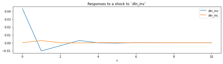
From the estimated VAR model, we can plot the impulse response functions of the endogenous variables.
[5]:
ax = res.impulse_responses(10, orthogonalized=True).plot(figsize=(13,3))
ax.set(xlabel='t', title='Responses to a shock to `dln_inv`');
[5]:
[Text(0.5, 0, 't'), Text(0.5, 1.0, 'Responses to a shock to `dln_inv`')]
Example 2: VMA
A vector moving average model can also be formulated. Below we show a VMA(2) on the same data, but where the innovations to the process are uncorrelated. In this example we leave out the exogenous regressor but now include the constant term.
[6]:
mod = sm.tsa.VARMAX(endog[['dln_inv', 'dln_inc']], order=(0,2), error_cov_type='diagonal')
res = mod.fit(maxiter=1000, disp=False)
print(res.summary())
                             Statespace Model Results
==================================================================================
Dep. Variable:     ['dln_inv', 'dln_inc']   No. Observations:                   75
Model:                             VMA(2)   Log Likelihood                 353.886
                              + intercept   AIC                           -683.771
Date:                    Tue, 02 Feb 2021   BIC                           -655.961
Time:                            06:54:27   HQIC                          -672.667
Sample:                        04-01-1960
                             - 10-01-1978
Covariance Type:                      opg
===================================================================================
Ljung-Box (L1) (Q):             0.01, 0.07   Jarque-Bera (JB):         12.35, 12.99
Prob(Q):                        0.93, 0.78   Prob(JB):                   0.00, 0.00
Heteroskedasticity (H):         0.44, 0.81   Skew:                      0.05, -0.48
Prob(H) (two-sided):            0.04, 0.60   Kurtosis:                   4.99, 4.80
                           Results for equation dln_inv
=================================================================================
                    coef    std err          z      P>|z|      [0.025      0.975]
---------------------------------------------------------------------------------
intercept         0.0182      0.005      3.824      0.000       0.009       0.028
L1.e(dln_inv)    -0.2620      0.106     -2.481      0.013      -0.469      -0.055
L1.e(dln_inc)     0.5405      0.633      0.854      0.393      -0.700       1.781
L2.e(dln_inv)     0.0298      0.148      0.201      0.841      -0.261       0.320
L2.e(dln_inc)     0.1630      0.477      0.341      0.733      -0.773       1.099
                           Results for equation dln_inc
=================================================================================
                    coef    std err          z      P>|z|      [0.025      0.975]
---------------------------------------------------------------------------------
intercept         0.0207      0.002     13.123      0.000       0.018       0.024
L1.e(dln_inv)     0.0489      0.041      1.178      0.239      -0.032       0.130
L1.e(dln_inc)    -0.0806      0.139     -0.580      0.562      -0.353       0.192
L2.e(dln_inv)     0.0174      0.042      0.410      0.682      -0.066       0.101
L2.e(dln_inc)     0.1278      0.152      0.842      0.400      -0.170       0.425
                             Error covariance matrix
==================================================================================
                     coef    std err          z      P>|z|      [0.025      0.975]
----------------------------------------------------------------------------------
sigma2.dln_inv     0.0020      0.000      7.344      0.000       0.001       0.003
sigma2.dln_inc     0.0001   2.32e-05      5.834      0.000    9.01e-05       0.000
==================================================================================

Warnings:
[1] Covariance matrix calculated using the outer product of gradients (complex-step).
/home/travis/build/statsmodels/statsmodels/statsmodels/base/model.py:568: ConvergenceWarning: Maximum Likelihood optimization failed to converge. Check mle_retvals
  ConvergenceWarning)
Caution: VARMA(p,q) specifications
Although the model allows estimating VARMA(p,q) specifications, these models are not identified without additional restrictions on the representation matrices, which are not built-in. For this reason, it is recommended that the user proceed with error (and indeed a warning is issued when these models are specified). Nonetheless, they may in some circumstances provide useful information.
[7]:
mod = sm.tsa.VARMAX(endog[['dln_inv', 'dln_inc']], order=(1,1))
res = mod.fit(maxiter=1000, disp=False)
print(res.summary())
/home/travis/build/statsmodels/statsmodels/statsmodels/tsa/statespace/varmax.py:163: EstimationWarning: Estimation of VARMA(p,q) models is not generically robust, due especially to identification issues.
  EstimationWarning)
                             Statespace Model Results
==================================================================================
Dep. Variable:     ['dln_inv', 'dln_inc']   No. Observations:                   75
Model:                         VARMA(1,1)   Log Likelihood                 354.287
                              + intercept   AIC                           -682.575
Date:                    Tue, 02 Feb 2021   BIC                           -652.448
Time:                            06:54:29   HQIC                          -670.545
Sample:                        04-01-1960
                             - 10-01-1978
Covariance Type:                      opg
===================================================================================
Ljung-Box (L1) (Q):             0.01, 0.06   Jarque-Bera (JB):         11.05, 14.18
Prob(Q):                        0.94, 0.81   Prob(JB):                   0.00, 0.00
Heteroskedasticity (H):         0.43, 0.91   Skew:                      0.01, -0.46
Prob(H) (two-sided):            0.04, 0.81   Kurtosis:                   4.88, 4.92
                           Results for equation dln_inv
=================================================================================
                    coef    std err          z      P>|z|      [0.025      0.975]
---------------------------------------------------------------------------------
intercept         0.0105      0.066      0.160      0.873      -0.118       0.139
L1.dln_inv       -0.0061      0.697     -0.009      0.993      -1.372       1.359
L1.dln_inc        0.3804      2.768      0.137      0.891      -5.044       5.805
L1.e(dln_inv)    -0.2487      0.707     -0.352      0.725      -1.635       1.138
L1.e(dln_inc)     0.1253      3.017      0.042      0.967      -5.788       6.038
                           Results for equation dln_inc
=================================================================================
                    coef    std err          z      P>|z|      [0.025      0.975]
---------------------------------------------------------------------------------
intercept         0.0165      0.027      0.601      0.548      -0.037       0.070
L1.dln_inv       -0.0336      0.278     -0.121      0.904      -0.579       0.512
L1.dln_inc        0.2349      1.117      0.210      0.833      -1.955       2.425
L1.e(dln_inv)     0.0888      0.285      0.312      0.755      -0.470       0.647
L1.e(dln_inc)    -0.2376      1.152     -0.206      0.837      -2.495       2.020
                                  Error covariance matrix
============================================================================================
                               coef    std err          z      P>|z|      [0.025      0.975]
--------------------------------------------------------------------------------------------
sqrt.var.dln_inv             0.0449      0.003     14.533      0.000       0.039       0.051
sqrt.cov.dln_inv.dln_inc     0.0017      0.003      0.649      0.516      -0.003       0.007
sqrt.var.dln_inc             0.0116      0.001     11.717      0.000       0.010       0.013
============================================================================================

Warnings:
[1] Covariance matrix calculated using the outer product of gradients (complex-step).