Prediction (out of sample)
[1]:
%matplotlib inline
[2]:
import numpy as np
import matplotlib.pyplot as plt

import statsmodels.api as sm

plt.rc("figure", figsize=(16, 8))
plt.rc("font", size=14)
Artificial data
[3]:
nsample = 50
sig = 0.25
x1 = np.linspace(0, 20, nsample)
X = np.column_stack((x1, np.sin(x1), (x1 - 5) ** 2))
X = sm.add_constant(X)
beta = [5.0, 0.5, 0.5, -0.02]
y_true = np.dot(X, beta)
y = y_true + sig * np.random.normal(size=nsample)
Estimation
[4]:
olsmod = sm.OLS(y, X)
olsres = olsmod.fit()
print(olsres.summary())
                            OLS Regression Results
==============================================================================
Dep. Variable:                      y   R-squared:                       0.986
Model:                            OLS   Adj. R-squared:                  0.985
Method:                 Least Squares   F-statistic:                     1095.
Date:                Fri, 05 May 2023   Prob (F-statistic):           9.24e-43
Time:                        13:46:30   Log-Likelihood:                 5.5153
No. Observations:                  50   AIC:                            -3.031
Df Residuals:                      46   BIC:                             4.618
Df Model:                           3
Covariance Type:            nonrobust
==============================================================================
                 coef    std err          t      P>|t|      [0.025      0.975]
------------------------------------------------------------------------------
const          5.1190      0.077     66.476      0.000       4.964       5.274
x1             0.4958      0.012     41.750      0.000       0.472       0.520
x2             0.4406      0.047      9.438      0.000       0.347       0.535
x3            -0.0198      0.001    -18.970      0.000      -0.022      -0.018
==============================================================================
Omnibus:                        0.463   Durbin-Watson:                   2.419
Prob(Omnibus):                  0.793   Jarque-Bera (JB):                0.179
Skew:                          -0.144   Prob(JB):                        0.915
Kurtosis:                       3.047   Cond. No.                         221.
==============================================================================

Notes:
[1] Standard Errors assume that the covariance matrix of the errors is correctly specified.
In-sample prediction
[5]:
ypred = olsres.predict(X)
print(ypred)
[ 4.62445026  5.0791561   5.49853785  5.85858285  6.14394448  6.35046358
  6.48585175  6.56842443  6.62409164  6.68210109  6.77023286  6.91023518
  7.1142513   7.38282436  7.70480816  8.05919845  8.41858387  8.75364956
  9.03799351  9.25246431  9.38830773  9.44860496  9.44776639  9.40916405
  9.36129162  9.33308304  9.34915868  9.42578035  9.5681795   9.76969769
 10.0128806  10.27234567 10.51895244 10.7245902  10.86679651 10.93244774
 10.91991521 10.8393328  10.71093198 10.56171783 10.42103219 10.31573286
 10.26578097 10.28096139 10.35927514 10.48726778 10.64223995 10.79597683
 10.91938372 10.98726625]
Create a new sample of explanatory variables Xnew, predict and plot
[6]:
x1n = np.linspace(20.5, 25, 10)
Xnew = np.column_stack((x1n, np.sin(x1n), (x1n - 5) ** 2))
Xnew = sm.add_constant(Xnew)
ynewpred = olsres.predict(Xnew)  # predict out of sample
print(ynewpred)
[10.97049523 10.83630035 10.60196055 10.3068523  10.00280887  9.74142978
  9.5614474   9.47924392  9.48484044  9.54434013]
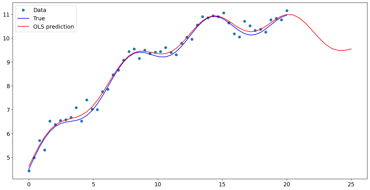
Plot comparison
[7]:
import matplotlib.pyplot as plt

fig, ax = plt.subplots()
ax.plot(x1, y, "o", label="Data")
ax.plot(x1, y_true, "b-", label="True")
ax.plot(np.hstack((x1, x1n)), np.hstack((ypred, ynewpred)), "r", label="OLS prediction")
ax.legend(loc="best")
[7]:
<matplotlib.legend.Legend at 0x7fceb3698a60>
Predicting with Formulas
Using formulas can make both estimation and prediction a lot easier
[8]:
from statsmodels.formula.api import ols

data = {"x1": x1, "y": y}

res = ols("y ~ x1 + np.sin(x1) + I((x1-5)**2)", data=data).fit()
We use the I to indicate use of the Identity transform. Ie., we do not want any expansion magic from using **2
[9]:
res.params
[9]:
Intercept           5.118951
x1                  0.495829
np.sin(x1)          0.440606
I((x1 - 5) ** 2)   -0.019780
dtype: float64
Now we only have to pass the single variable and we get the transformed right-hand side variables automatically
[10]:
res.predict(exog=dict(x1=x1n))
[10]:
0    10.970495
1    10.836300
2    10.601961
3    10.306852
4    10.002809
5     9.741430
6     9.561447
7     9.479244
8     9.484840
9     9.544340
dtype: float64
Last update:
May 05, 2023