Prediction (out of sample)
[1]:
%matplotlib inline
[2]:
import numpy as np
import matplotlib.pyplot as plt

import statsmodels.api as sm

plt.rc("figure", figsize=(16, 8))
plt.rc("font", size=14)
Artificial data
[3]:
nsample = 50
sig = 0.25
x1 = np.linspace(0, 20, nsample)
X = np.column_stack((x1, np.sin(x1), (x1 - 5) ** 2))
X = sm.add_constant(X)
beta = [5.0, 0.5, 0.5, -0.02]
y_true = np.dot(X, beta)
y = y_true + sig * np.random.normal(size=nsample)
Estimation
[4]:
olsmod = sm.OLS(y, X)
olsres = olsmod.fit()
print(olsres.summary())
                            OLS Regression Results
==============================================================================
Dep. Variable:                      y   R-squared:                       0.982
Model:                            OLS   Adj. R-squared:                  0.980
Method:                 Least Squares   F-statistic:                     814.3
Date:                Mon, 16 Sep 2024   Prob (F-statistic):           7.44e-40
Time:                        10:18:29   Log-Likelihood:               -0.96901
No. Observations:                  50   AIC:                             9.938
Df Residuals:                      46   BIC:                             17.59
Df Model:                           3
Covariance Type:            nonrobust
==============================================================================
                 coef    std err          t      P>|t|      [0.025      0.975]
------------------------------------------------------------------------------
const          5.0679      0.088     57.808      0.000       4.891       5.244
x1             0.4917      0.014     36.368      0.000       0.464       0.519
x2             0.4194      0.053      7.890      0.000       0.312       0.526
x3            -0.0200      0.001    -16.858      0.000      -0.022      -0.018
==============================================================================
Omnibus:                        1.967   Durbin-Watson:                   1.883
Prob(Omnibus):                  0.374   Jarque-Bera (JB):                1.621
Skew:                          -0.439   Prob(JB):                        0.445
Kurtosis:                       2.923   Cond. No.                         221.
==============================================================================

Notes:
[1] Standard Errors assume that the covariance matrix of the errors is correctly specified.
In-sample prediction
[5]:
ypred = olsres.predict(X)
print(ypred)
[ 4.56757354  5.01307964  5.42456918  5.77918693  6.062326    6.27002771
  6.40963196  6.49857135  6.56150701  6.62627688  6.71932199  6.86134231
  7.06389575  7.32749927  7.64154393  7.98603792  8.33489113  8.66020171
  8.93684026  9.14657851  9.28108417  9.34328992  9.34691156  9.31419455
  9.27225916  9.24864465  9.26678467  9.3421572   9.47974151  9.67320013
  9.90592004 10.15374216 10.38893063 10.5847297  10.71975967 10.78152947
 10.76848892 10.69028344 10.56616933 10.42184998 10.28525291 10.18194136
 10.1309143  10.14148497 10.21175072 10.32890564 10.47134452 10.61221251
 10.72381732 10.78217898]
Create a new sample of explanatory variables Xnew, predict and plot
[6]:
x1n = np.linspace(20.5, 25, 10)
Xnew = np.column_stack((x1n, np.sin(x1n), (x1n - 5) ** 2))
Xnew = sm.add_constant(Xnew)
ynewpred = olsres.predict(Xnew)  # predict out of sample
print(ynewpred)
[10.758023   10.62151019 10.38908661 10.09823073  9.79827743  9.53833904
  9.35528098  9.26469583  9.25708566  9.3001875 ]
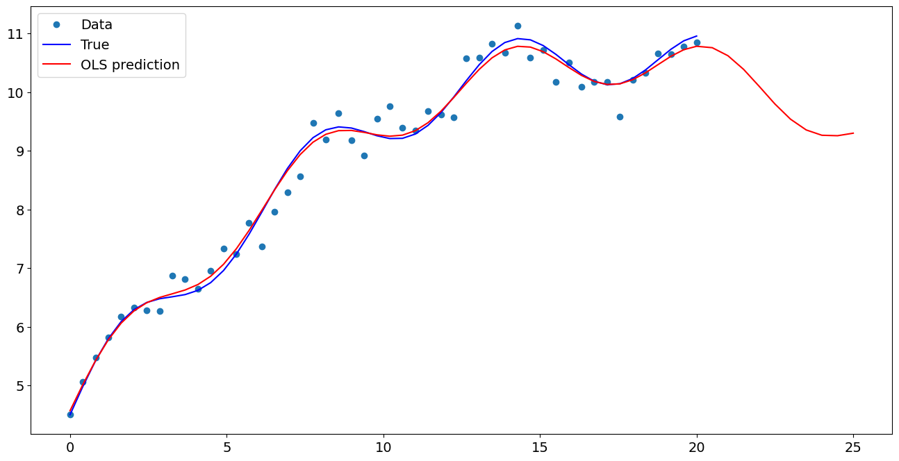
Plot comparison
[7]:
import matplotlib.pyplot as plt

fig, ax = plt.subplots()
ax.plot(x1, y, "o", label="Data")
ax.plot(x1, y_true, "b-", label="True")
ax.plot(np.hstack((x1, x1n)), np.hstack((ypred, ynewpred)), "r", label="OLS prediction")
ax.legend(loc="best")
[7]:
<matplotlib.legend.Legend at 0x7f17b0aa3eb0>
Predicting with Formulas
Using formulas can make both estimation and prediction a lot easier
[8]:
from statsmodels.formula.api import ols

data = {"x1": x1, "y": y}

res = ols("y ~ x1 + np.sin(x1) + I((x1-5)**2)", data=data).fit()
We use the I to indicate use of the Identity transform. Ie., we do not want any expansion magic from using **2
[9]:
res.params
[9]:
Intercept           5.067886
x1                  0.491712
np.sin(x1)          0.419369
I((x1 - 5) ** 2)   -0.020013
dtype: float64
Now we only have to pass the single variable and we get the transformed right-hand side variables automatically
[10]:
res.predict(exog=dict(x1=x1n))
[10]:
0    10.758023
1    10.621510
2    10.389087
3    10.098231
4     9.798277
5     9.538339
6     9.355281
7     9.264696
8     9.257086
9     9.300188
dtype: float64
Last update:
Sep 16, 2024