Robust Linear Models
[1]:
%matplotlib inline
[2]:
import matplotlib.pyplot as plt
import numpy as np
import statsmodels.api as sm
Estimation
Load data:
[3]:
data = sm.datasets.stackloss.load()
data.exog = sm.add_constant(data.exog)
Huber’s T norm with the (default) median absolute deviation scaling
[4]:
huber_t = sm.RLM(data.endog, data.exog, M=sm.robust.norms.HuberT())
hub_results = huber_t.fit()
print(hub_results.params)
print(hub_results.bse)
print(
    hub_results.summary(
        yname="y", xname=["var_%d" % i for i in range(len(hub_results.params))]
    )
)
const       -41.026498
AIRFLOW       0.829384
WATERTEMP     0.926066
ACIDCONC     -0.127847
dtype: float64
const        9.791899
AIRFLOW      0.111005
WATERTEMP    0.302930
ACIDCONC     0.128650
dtype: float64
                    Robust linear Model Regression Results
==============================================================================
Dep. Variable:                      y   No. Observations:                   21
Model:                            RLM   Df Residuals:                       17
Method:                          IRLS   Df Model:                            3
Norm:                          HuberT
Scale Est.:                       mad
Cov Type:                          H1
Date:                Mon, 16 Sep 2024
Time:                        09:59:09
No. Iterations:                    19
==============================================================================
                 coef    std err          z      P>|z|      [0.025      0.975]
------------------------------------------------------------------------------
var_0        -41.0265      9.792     -4.190      0.000     -60.218     -21.835
var_1          0.8294      0.111      7.472      0.000       0.612       1.047
var_2          0.9261      0.303      3.057      0.002       0.332       1.520
var_3         -0.1278      0.129     -0.994      0.320      -0.380       0.124
==============================================================================

If the model instance has been used for another fit with different fit parameters, then the fit options might not be the correct ones anymore .
Huber’s T norm with ‘H2’ covariance matrix
[5]:
hub_results2 = huber_t.fit(cov="H2")
print(hub_results2.params)
print(hub_results2.bse)
const       -41.026498
AIRFLOW       0.829384
WATERTEMP     0.926066
ACIDCONC     -0.127847
dtype: float64
const        9.089504
AIRFLOW      0.119460
WATERTEMP    0.322355
ACIDCONC     0.117963
dtype: float64
Andrew’s Wave norm with Huber’s Proposal 2 scaling and ‘H3’ covariance matrix
[6]:
andrew_mod = sm.RLM(data.endog, data.exog, M=sm.robust.norms.AndrewWave())
andrew_results = andrew_mod.fit(scale_est=sm.robust.scale.HuberScale(), cov="H3")
print("Parameters: ", andrew_results.params)
Parameters:  const       -40.881796
AIRFLOW       0.792761
WATERTEMP     1.048576
ACIDCONC     -0.133609
dtype: float64
See help(sm.RLM.fit) for more options and module sm.robust.scale for scale options
Comparing OLS and RLM
Artificial data with outliers:
[7]:
nsample = 50
x1 = np.linspace(0, 20, nsample)
X = np.column_stack((x1, (x1 - 5) ** 2))
X = sm.add_constant(X)
sig = 0.3  # smaller error variance makes OLS<->RLM contrast bigger
beta = [5, 0.5, -0.0]
y_true2 = np.dot(X, beta)
y2 = y_true2 + sig * 1.0 * np.random.normal(size=nsample)
y2[[39, 41, 43, 45, 48]] -= 5  # add some outliers (10% of nsample)
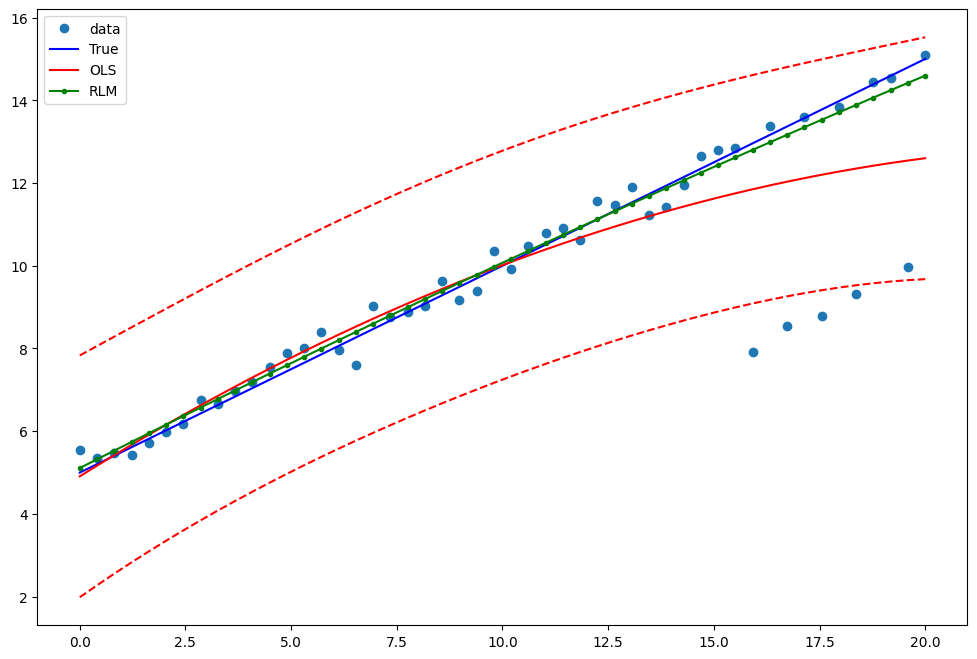
Example 1: quadratic function with linear truth
Note that the quadratic term in OLS regression will capture outlier effects.
[8]:
res = sm.OLS(y2, X).fit()
print(res.params)
print(res.bse)
print(res.predict())
[ 5.22421003  0.51052925 -0.01260019]
[0.44913658 0.06934063 0.00613558]
[ 4.9092053   5.16691477  5.42042593  5.66973877  5.9148533   6.15576952
  6.39248742  6.62500701  6.85332828  7.07745124  7.29737589  7.51310222
  7.72463024  7.93195995  8.13509134  8.33402442  8.52875918  8.71929564
  8.90563377  9.0877736   9.26571511  9.4394583   9.60900318  9.77434975
  9.93549801 10.09244795 10.24519958 10.39375289 10.53810789 10.67826458
 10.81422295 10.94598301 11.07354475 11.19690819 11.3160733  11.43104011
 11.5418086  11.64837878 11.75075064 11.84892419 11.94289942 12.03267635
 12.11825495 12.19963525 12.27681723 12.3498009  12.41858625 12.48317329
 12.54356201 12.59975243]
Estimate RLM:
[9]:
resrlm = sm.RLM(y2, X).fit()
print(resrlm.params)
print(resrlm.bse)
[ 5.16404489e+00  4.96217408e-01 -2.18756978e-03]
[0.129871   0.02005033 0.00177414]
Draw a plot to compare OLS estimates to the robust estimates:
[10]:
fig = plt.figure(figsize=(12, 8))
ax = fig.add_subplot(111)
ax.plot(x1, y2, "o", label="data")
ax.plot(x1, y_true2, "b-", label="True")
pred_ols = res.get_prediction()
iv_l = pred_ols.summary_frame()["obs_ci_lower"]
iv_u = pred_ols.summary_frame()["obs_ci_upper"]

ax.plot(x1, res.fittedvalues, "r-", label="OLS")
ax.plot(x1, iv_u, "r--")
ax.plot(x1, iv_l, "r--")
ax.plot(x1, resrlm.fittedvalues, "g.-", label="RLM")
ax.legend(loc="best")
[10]:
<matplotlib.legend.Legend at 0x7fc42cc63070>
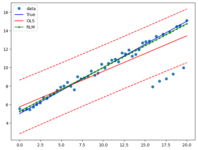
Example 2: linear function with linear truth
Fit a new OLS model using only the linear term and the constant:
[11]:
X2 = X[:, [0, 1]]
res2 = sm.OLS(y2, X2).fit()
print(res2.params)
print(res2.bse)
[5.73207479 0.38452736]
[0.3872825  0.03336983]
Estimate RLM:
[12]:
resrlm2 = sm.RLM(y2, X2).fit()
print(resrlm2.params)
print(resrlm2.bse)
[5.24713098 0.47452003]
[0.11089278 0.00955497]
Draw a plot to compare OLS estimates to the robust estimates:
[13]:
pred_ols = res2.get_prediction()
iv_l = pred_ols.summary_frame()["obs_ci_lower"]
iv_u = pred_ols.summary_frame()["obs_ci_upper"]

fig, ax = plt.subplots(figsize=(8, 6))
ax.plot(x1, y2, "o", label="data")
ax.plot(x1, y_true2, "b-", label="True")
ax.plot(x1, res2.fittedvalues, "r-", label="OLS")
ax.plot(x1, iv_u, "r--")
ax.plot(x1, iv_l, "r--")
ax.plot(x1, resrlm2.fittedvalues, "g.-", label="RLM")
legend = ax.legend(loc="best")
Last update:
Sep 16, 2024