Regression diagnostics
This example file shows how to use a few of the statsmodels regression diagnostic tests in a real-life context. You can learn about more tests and find out more information about the tests here on the Regression Diagnostics page.
Note that most of the tests described here only return a tuple of numbers, without any annotation. A full description of outputs is always included in the docstring and in the online statsmodels documentation. For presentation purposes, we use the zip(name,test) construct to pretty-print short descriptions in the examples below.
Estimate a regression model
[1]:
%matplotlib inline
[2]:
from statsmodels.compat import lzip

import numpy as np
import pandas as pd
import statsmodels.formula.api as smf
import statsmodels.stats.api as sms
import matplotlib.pyplot as plt

# Load data
url = "https://raw.githubusercontent.com/vincentarelbundock/Rdatasets/master/csv/HistData/Guerry.csv"
dat = pd.read_csv(url)

# Fit regression model (using the natural log of one of the regressors)
results = smf.ols("Lottery ~ Literacy + np.log(Pop1831)", data=dat).fit()

# Inspect the results
print(results.summary())
                            OLS Regression Results
==============================================================================
Dep. Variable:                Lottery   R-squared:                       0.348
Model:                            OLS   Adj. R-squared:                  0.333
Method:                 Least Squares   F-statistic:                     22.20
Date:                Fri, 05 Dec 2025   Prob (F-statistic):           1.90e-08
Time:                        18:10:32   Log-Likelihood:                -379.82
No. Observations:                  86   AIC:                             765.6
Df Residuals:                      83   BIC:                             773.0
Df Model:                           2
Covariance Type:            nonrobust
===================================================================================
                      coef    std err          t      P>|t|      [0.025      0.975]
-----------------------------------------------------------------------------------
Intercept         246.4341     35.233      6.995      0.000     176.358     316.510
Literacy           -0.4889      0.128     -3.832      0.000      -0.743      -0.235
np.log(Pop1831)   -31.3114      5.977     -5.239      0.000     -43.199     -19.424
==============================================================================
Omnibus:                        3.713   Durbin-Watson:                   2.019
Prob(Omnibus):                  0.156   Jarque-Bera (JB):                3.394
Skew:                          -0.487   Prob(JB):                        0.183
Kurtosis:                       3.003   Cond. No.                         702.
==============================================================================

Notes:
[1] Standard Errors assume that the covariance matrix of the errors is correctly specified.
Normality of the residuals
Jarque-Bera test:
[3]:
name = ["Jarque-Bera", "Chi^2 two-tail prob.", "Skew", "Kurtosis"]
test = sms.jarque_bera(results.resid)
lzip(name, test)
[3]:
[('Jarque-Bera', np.float64(3.39360802484318)),
 ('Chi^2 two-tail prob.', np.float64(0.18326831231663254)),
 ('Skew', np.float64(-0.4865803431122347)),
 ('Kurtosis', np.float64(3.003417757881634))]
Omni test:
[4]:
name = ["Chi^2", "Two-tail probability"]
test = sms.omni_normtest(results.resid)
lzip(name, test)
[4]:
[('Chi^2', np.float64(3.7134378115971933)),
 ('Two-tail probability', np.float64(0.15618424580304735))]
Influence tests
Once created, an object of class OLSInfluence holds attributes and methods that allow users to assess the influence of each observation. For example, we can compute and extract the first few rows of DFbetas by:
[5]:
from statsmodels.stats.outliers_influence import OLSInfluence

test_class = OLSInfluence(results)
test_class.dfbetas[:5, :]
[5]:
array([[-0.00301154,  0.00290872,  0.00118179],
       [-0.06425662,  0.04043093,  0.06281609],
       [ 0.01554894, -0.03556038, -0.00905336],
       [ 0.17899858,  0.04098207, -0.18062352],
       [ 0.29679073,  0.21249207, -0.3213655 ]])
Explore other options by typing dir(influence_test)
Useful information on leverage can also be plotted:
[6]:
from statsmodels.graphics.regressionplots import plot_leverage_resid2

fig, ax = plt.subplots(figsize=(8, 6))
fig = plot_leverage_resid2(results, ax=ax)
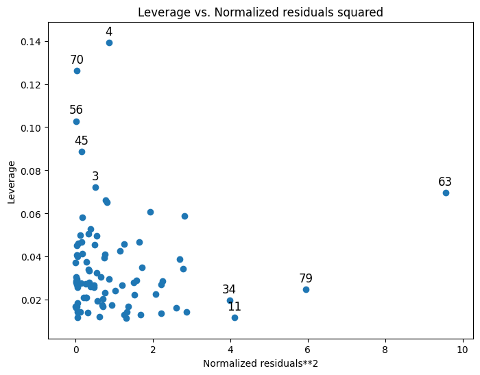
Other plotting options can be found on the Graphics page.
Multicollinearity
Condition number:
[7]:
np.linalg.cond(results.model.exog)
[7]:
np.float64(702.1792145490066)
Heteroskedasticity tests
Breush-Pagan test:
[8]:
name = ["Lagrange multiplier statistic", "p-value", "f-value", "f p-value"]
test = sms.het_breuschpagan(results.resid, results.model.exog)
lzip(name, test)
[8]:
[('Lagrange multiplier statistic', np.float64(4.893213374094005)),
 ('p-value', np.float64(0.08658690502352002)),
 ('f-value', np.float64(2.5037159462564618)),
 ('f p-value', np.float64(0.08794028782672814))]
Goldfeld-Quandt test
[9]:
name = ["F statistic", "p-value"]
test = sms.het_goldfeldquandt(results.resid, results.model.exog)
lzip(name, test)
[9]:
[('F statistic', np.float64(1.1002422436378143)),
 ('p-value', np.float64(0.38202950686925324))]
Linearity
Harvey-Collier multiplier test for Null hypothesis that the linear specification is correct:
[10]:
name = ["t value", "p value"]
test = sms.linear_harvey_collier(results)
lzip(name, test)
[10]:
[('t value', np.float64(-1.0796490077759802)),
 ('p value', np.float64(0.2834639247569222))]