Quasi-binomial regression
This notebook demonstrates using custom variance functions and non-binary data with the quasi-binomial GLM family to perform a regression analysis using a dependent variable that is a proportion.
The notebook uses the barley leaf blotch data that has been discussed in several textbooks. See below for one reference:
[1]:
import statsmodels.api as sm
import numpy as np
import pandas as pd
import matplotlib.pyplot as plt
from io import StringIO
The raw data, expressed as percentages. We will divide by 100 to obtain proportions.
[2]:
raw = StringIO(
    """0.05,0.00,1.25,2.50,5.50,1.00,5.00,5.00,17.50
0.00,0.05,1.25,0.50,1.00,5.00,0.10,10.00,25.00
0.00,0.05,2.50,0.01,6.00,5.00,5.00,5.00,42.50
0.10,0.30,16.60,3.00,1.10,5.00,5.00,5.00,50.00
0.25,0.75,2.50,2.50,2.50,5.00,50.00,25.00,37.50
0.05,0.30,2.50,0.01,8.00,5.00,10.00,75.00,95.00
0.50,3.00,0.00,25.00,16.50,10.00,50.00,50.00,62.50
1.30,7.50,20.00,55.00,29.50,5.00,25.00,75.00,95.00
1.50,1.00,37.50,5.00,20.00,50.00,50.00,75.00,95.00
1.50,12.70,26.25,40.00,43.50,75.00,75.00,75.00,95.00"""
)
The regression model is a two-way additive model with site and variety effects. The data are a full unreplicated design with 10 rows (sites) and 9 columns (varieties).
[3]:
df = pd.read_csv(raw, header=None)
df = df.melt()
df["site"] = 1 + np.floor(df.index / 10).astype(int)
df["variety"] = 1 + (df.index % 10)
df = df.rename(columns={"value": "blotch"})
df = df.drop("variable", axis=1)
df["blotch"] /= 100
Fit the quasi-binomial regression with the standard variance function.
[4]:
model1 = sm.GLM.from_formula(
    "blotch ~ 0 + C(variety) + C(site)", family=sm.families.Binomial(), data=df
)
result1 = model1.fit(scale="X2")
print(result1.summary())
                 Generalized Linear Model Regression Results
==============================================================================
Dep. Variable:                 blotch   No. Observations:                   90
Model:                            GLM   Df Residuals:                       72
Model Family:                Binomial   Df Model:                           17
Link Function:                  Logit   Scale:                        0.088778
Method:                          IRLS   Log-Likelihood:                -20.791
Date:                Sun, 14 Jun 2026   Deviance:                       6.1260
Time:                        16:00:10   Pearson chi2:                     6.39
No. Iterations:                    10   Pseudo R-squ. (CS):             0.3198
Covariance Type:            nonrobust
==================================================================================
                     coef    std err          z      P>|z|      [0.025      0.975]
----------------------------------------------------------------------------------
C(variety)[1]     -8.0546      1.422     -5.664      0.000     -10.842      -5.268
C(variety)[2]     -7.9046      1.412     -5.599      0.000     -10.672      -5.138
C(variety)[3]     -7.3652      1.384     -5.321      0.000     -10.078      -4.652
C(variety)[4]     -7.0065      1.372     -5.109      0.000      -9.695      -4.318
C(variety)[5]     -6.4399      1.357     -4.746      0.000      -9.100      -3.780
C(variety)[6]     -5.6835      1.344     -4.230      0.000      -8.317      -3.050
C(variety)[7]     -5.4841      1.341     -4.090      0.000      -8.112      -2.856
C(variety)[8]     -4.7126      1.331     -3.539      0.000      -7.322      -2.103
C(variety)[9]     -4.5546      1.330     -3.425      0.001      -7.161      -1.948
C(variety)[10]    -3.8016      1.320     -2.881      0.004      -6.388      -1.215
C(site)[T.2]       1.6391      1.443      1.136      0.256      -1.190       4.468
C(site)[T.3]       3.3265      1.349      2.466      0.014       0.682       5.971
C(site)[T.4]       3.5822      1.344      2.664      0.008       0.947       6.217
C(site)[T.5]       3.5831      1.344      2.665      0.008       0.948       6.218
C(site)[T.6]       3.8933      1.340      2.905      0.004       1.266       6.520
C(site)[T.7]       4.7300      1.335      3.544      0.000       2.114       7.346
C(site)[T.8]       5.5227      1.335      4.138      0.000       2.907       8.139
C(site)[T.9]       6.7946      1.341      5.068      0.000       4.167       9.422
==================================================================================
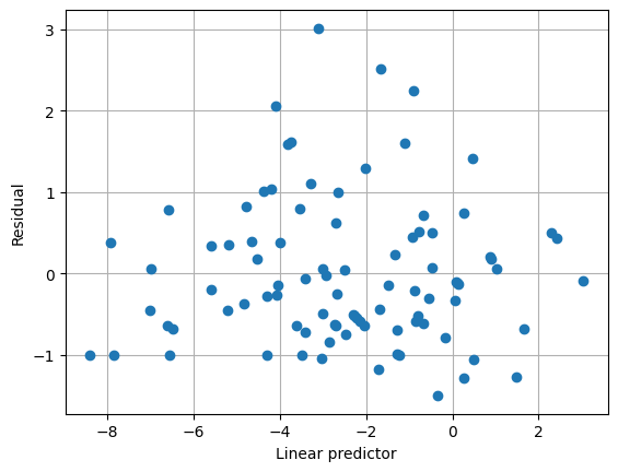
The plot below shows that the default variance function is not capturing the variance structure very well. Also note that the scale parameter estimate is quite small.
[5]:
plt.clf()
plt.grid(True)
plt.plot(result1.predict(linear=True), result1.resid_pearson, "o")
plt.xlabel("Linear predictor")
plt.ylabel("Residual")
/opt/hostedtoolcache/Python/3.10.20/x64/lib/python3.10/site-packages/statsmodels/base/model.py:1256: FutureWarning: linear keyword is deprecated, use which="linear"
  predict_results = self.model.predict(self.params, exog, *args, **kwargs)
[5]:
Text(0, 0.5, 'Residual')
An alternative variance function is mu^2 * (1 - mu)^2.
[6]:
class vf(sm.families.varfuncs.VarianceFunction):
    def __call__(self, mu):
        return mu**2 * (1 - mu) ** 2

    def deriv(self, mu):
        return 2 * mu - 6 * mu**2 + 4 * mu**3
Fit the quasi-binomial regression with the alternative variance function.
[7]:
bin = sm.families.Binomial()
bin.variance = vf()
model2 = sm.GLM.from_formula("blotch ~ 0 + C(variety) + C(site)", family=bin, data=df)
result2 = model2.fit(scale="X2")
print(result2.summary())
                 Generalized Linear Model Regression Results
==============================================================================
Dep. Variable:                 blotch   No. Observations:                   90
Model:                            GLM   Df Residuals:                       72
Model Family:                Binomial   Df Model:                           17
Link Function:                  Logit   Scale:                         0.98855
Method:                          IRLS   Log-Likelihood:                -21.335
Date:                Sun, 14 Jun 2026   Deviance:                       7.2134
Time:                        16:00:10   Pearson chi2:                     71.2
No. Iterations:                    25   Pseudo R-squ. (CS):             0.3115
Covariance Type:            nonrobust
==================================================================================
                     coef    std err          z      P>|z|      [0.025      0.975]
----------------------------------------------------------------------------------
C(variety)[1]     -7.9224      0.445    -17.817      0.000      -8.794      -7.051
C(variety)[2]     -8.3897      0.445    -18.868      0.000      -9.261      -7.518
C(variety)[3]     -7.8436      0.445    -17.640      0.000      -8.715      -6.972
C(variety)[4]     -6.9683      0.445    -15.672      0.000      -7.840      -6.097
C(variety)[5]     -6.5697      0.445    -14.775      0.000      -7.441      -5.698
C(variety)[6]     -6.5938      0.445    -14.829      0.000      -7.465      -5.722
C(variety)[7]     -5.5823      0.445    -12.555      0.000      -6.454      -4.711
C(variety)[8]     -4.6598      0.445    -10.480      0.000      -5.531      -3.788
C(variety)[9]     -4.7869      0.445    -10.766      0.000      -5.658      -3.915
C(variety)[10]    -4.0351      0.445     -9.075      0.000      -4.907      -3.164
C(site)[T.2]       1.3831      0.445      3.111      0.002       0.512       2.255
C(site)[T.3]       3.8601      0.445      8.681      0.000       2.989       4.732
C(site)[T.4]       3.5570      0.445      8.000      0.000       2.686       4.428
C(site)[T.5]       4.1079      0.445      9.239      0.000       3.236       4.979
C(site)[T.6]       4.3054      0.445      9.683      0.000       3.434       5.177
C(site)[T.7]       4.9181      0.445     11.061      0.000       4.047       5.790
C(site)[T.8]       5.6949      0.445     12.808      0.000       4.823       6.566
C(site)[T.9]       7.0676      0.445     15.895      0.000       6.196       7.939
==================================================================================
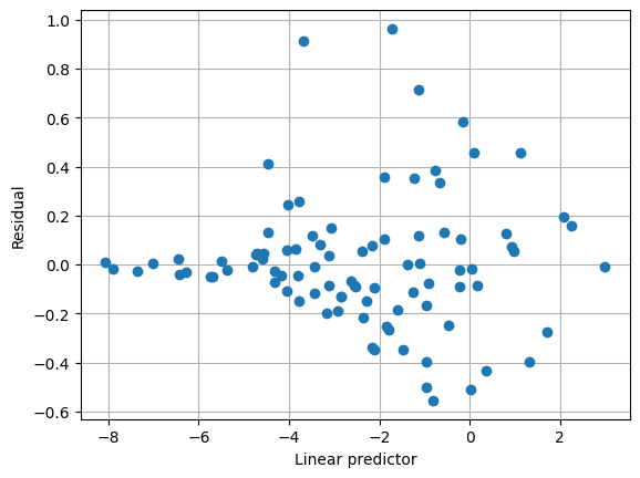
With the alternative variance function, the mean/variance relationship seems to capture the data well, and the estimated scale parameter is close to 1.
[8]:
plt.clf()
plt.grid(True)
plt.plot(result2.predict(linear=True), result2.resid_pearson, "o")
plt.xlabel("Linear predictor")
plt.ylabel("Residual")
/opt/hostedtoolcache/Python/3.10.20/x64/lib/python3.10/site-packages/statsmodels/base/model.py:1256: FutureWarning: linear keyword is deprecated, use which="linear"
  predict_results = self.model.predict(self.params, exog, *args, **kwargs)
[8]:
Text(0, 0.5, 'Residual')