Deterministic Terms in Time Series Models¶

[1]:

import matplotlib.pyplot as plt
import numpy as np
import pandas as pd

plt.rc("figure", figsize=(16, 9))
plt.rc("font", size=16)

Basic Use¶

Basic configurations can be directly constructed through DeterministicProcess. These can include a constant, a time trend of any order, and either a seasonal or a Fourier component.

The process requires an index, which is the index of the full-sample (or in-sample).

First, we initialize a deterministic process with a constant, a linear time trend, and a 5-period seasonal term. The in_sample method returns the full set of values that match the index.

[2]:

from statsmodels.tsa.deterministic import DeterministicProcess

index = pd.RangeIndex(0, 100)
det_proc = DeterministicProcess(index, constant=True, order=1, seasonal=True, period=5)
det_proc.in_sample()

[2]:

	const	trend	s(2,5)	s(3,5)	s(4,5)	s(5,5)
0	1.0	1.0	0.0	0.0	0.0	0.0
1	1.0	2.0	1.0	0.0	0.0	0.0
2	1.0	3.0	0.0	1.0	0.0	0.0
3	1.0	4.0	0.0	0.0	1.0	0.0
4	1.0	5.0	0.0	0.0	0.0	1.0
...	...	...	...	...	...	...
95	1.0	96.0	0.0	0.0	0.0	0.0
96	1.0	97.0	1.0	0.0	0.0	0.0
97	1.0	98.0	0.0	1.0	0.0	0.0
98	1.0	99.0	0.0	0.0	1.0	0.0
99	1.0	100.0	0.0	0.0	0.0	1.0

100 rows × 6 columns

The out_of_sample returns the next steps values after the end of the in-sample.

[3]:

det_proc.out_of_sample(15)

[3]:

	const	trend	s(2,5)	s(3,5)	s(4,5)	s(5,5)
100	1.0	101.0	0.0	0.0	0.0	0.0
101	1.0	102.0	1.0	0.0	0.0	0.0
102	1.0	103.0	0.0	1.0	0.0	0.0
103	1.0	104.0	0.0	0.0	1.0	0.0
104	1.0	105.0	0.0	0.0	0.0	1.0
105	1.0	106.0	0.0	0.0	0.0	0.0
106	1.0	107.0	1.0	0.0	0.0	0.0
107	1.0	108.0	0.0	1.0	0.0	0.0
108	1.0	109.0	0.0	0.0	1.0	0.0
109	1.0	110.0	0.0	0.0	0.0	1.0
110	1.0	111.0	0.0	0.0	0.0	0.0
111	1.0	112.0	1.0	0.0	0.0	0.0
112	1.0	113.0	0.0	1.0	0.0	0.0
113	1.0	114.0	0.0	0.0	1.0	0.0
114	1.0	115.0	0.0	0.0	0.0	1.0

range(start, stop) can also be used to produce the deterministic terms over any range including in- and out-of-sample.

Notes¶

When the index is a pandas DatetimeIndex or a PeriodIndex, then start and stop can be date-like (strings, e.g., “2020-06-01”, or Timestamp) or integers.
stop is always included in the range. While this is not very Pythonic, it is needed since both statsmodels and Pandas include stop when working with date-like slices.

[4]:

det_proc.range(190, 210)

[4]:

	const	trend	s(2,5)	s(3,5)	s(4,5)	s(5,5)
190	1.0	191.0	0.0	0.0	0.0	0.0
191	1.0	192.0	1.0	0.0	0.0	0.0
192	1.0	193.0	0.0	1.0	0.0	0.0
193	1.0	194.0	0.0	0.0	1.0	0.0
194	1.0	195.0	0.0	0.0	0.0	1.0
195	1.0	196.0	0.0	0.0	0.0	0.0
196	1.0	197.0	1.0	0.0	0.0	0.0
197	1.0	198.0	0.0	1.0	0.0	0.0
198	1.0	199.0	0.0	0.0	1.0	0.0
199	1.0	200.0	0.0	0.0	0.0	1.0
200	1.0	201.0	0.0	0.0	0.0	0.0
201	1.0	202.0	1.0	0.0	0.0	0.0
202	1.0	203.0	0.0	1.0	0.0	0.0
203	1.0	204.0	0.0	0.0	1.0	0.0
204	1.0	205.0	0.0	0.0	0.0	1.0
205	1.0	206.0	0.0	0.0	0.0	0.0
206	1.0	207.0	1.0	0.0	0.0	0.0
207	1.0	208.0	0.0	1.0	0.0	0.0
208	1.0	209.0	0.0	0.0	1.0	0.0
209	1.0	210.0	0.0	0.0	0.0	1.0
210	1.0	211.0	0.0	0.0	0.0	0.0

Using a Date-like Index¶

Next, we show the same steps using a PeriodIndex.

[5]:

index = pd.period_range("2020-03-01", freq="M", periods=60)
det_proc = DeterministicProcess(index, constant=True, fourier=2)
det_proc.in_sample().head(12)

[5]:

	const	sin(1,12)	cos(1,12)	sin(2,12)	cos(2,12)
2020-03	1.0	0.000000e+00	1.000000e+00	0.000000e+00	1.0
2020-04	1.0	5.000000e-01	8.660254e-01	8.660254e-01	0.5
2020-05	1.0	8.660254e-01	5.000000e-01	8.660254e-01	-0.5
2020-06	1.0	1.000000e+00	6.123234e-17	1.224647e-16	-1.0
2020-07	1.0	8.660254e-01	-5.000000e-01	-8.660254e-01	-0.5
2020-08	1.0	5.000000e-01	-8.660254e-01	-8.660254e-01	0.5
2020-09	1.0	1.224647e-16	-1.000000e+00	-2.449294e-16	1.0
2020-10	1.0	-5.000000e-01	-8.660254e-01	8.660254e-01	0.5
2020-11	1.0	-8.660254e-01	-5.000000e-01	8.660254e-01	-0.5
2020-12	1.0	-1.000000e+00	-1.836970e-16	3.673940e-16	-1.0
2021-01	1.0	-8.660254e-01	5.000000e-01	-8.660254e-01	-0.5
2021-02	1.0	-5.000000e-01	8.660254e-01	-8.660254e-01	0.5

[6]:

det_proc.out_of_sample(12)

[6]:

	const	sin(1,12)	cos(1,12)	sin(2,12)	cos(2,12)
2025-03	1.0	-1.224647e-15	1.000000e+00	-2.449294e-15	1.0
2025-04	1.0	5.000000e-01	8.660254e-01	8.660254e-01	0.5
2025-05	1.0	8.660254e-01	5.000000e-01	8.660254e-01	-0.5
2025-06	1.0	1.000000e+00	-4.904777e-16	-9.809554e-16	-1.0
2025-07	1.0	8.660254e-01	-5.000000e-01	-8.660254e-01	-0.5
2025-08	1.0	5.000000e-01	-8.660254e-01	-8.660254e-01	0.5
2025-09	1.0	4.899825e-15	-1.000000e+00	-9.799650e-15	1.0
2025-10	1.0	-5.000000e-01	-8.660254e-01	8.660254e-01	0.5
2025-11	1.0	-8.660254e-01	-5.000000e-01	8.660254e-01	-0.5
2025-12	1.0	-1.000000e+00	-3.184701e-15	6.369401e-15	-1.0
2026-01	1.0	-8.660254e-01	5.000000e-01	-8.660254e-01	-0.5
2026-02	1.0	-5.000000e-01	8.660254e-01	-8.660254e-01	0.5

range accepts date-like arguments, which are usually given as strings.

[7]:

det_proc.range("2025-01", "2026-01")

[7]:

	const	sin(1,12)	cos(1,12)	sin(2,12)	cos(2,12)
2025-01	1.0	-8.660254e-01	5.000000e-01	-8.660254e-01	-0.5
2025-02	1.0	-5.000000e-01	8.660254e-01	-8.660254e-01	0.5
2025-03	1.0	-1.224647e-15	1.000000e+00	-2.449294e-15	1.0
2025-04	1.0	5.000000e-01	8.660254e-01	8.660254e-01	0.5
2025-05	1.0	8.660254e-01	5.000000e-01	8.660254e-01	-0.5
2025-06	1.0	1.000000e+00	-4.904777e-16	-9.809554e-16	-1.0
2025-07	1.0	8.660254e-01	-5.000000e-01	-8.660254e-01	-0.5
2025-08	1.0	5.000000e-01	-8.660254e-01	-8.660254e-01	0.5
2025-09	1.0	4.899825e-15	-1.000000e+00	-9.799650e-15	1.0
2025-10	1.0	-5.000000e-01	-8.660254e-01	8.660254e-01	0.5
2025-11	1.0	-8.660254e-01	-5.000000e-01	8.660254e-01	-0.5
2025-12	1.0	-1.000000e+00	-3.184701e-15	6.369401e-15	-1.0
2026-01	1.0	-8.660254e-01	5.000000e-01	-8.660254e-01	-0.5

This is equivalent to using the integer values 58 and 70.

[8]:

det_proc.range(58, 70)

[8]:

	const	sin(1,12)	cos(1,12)	sin(2,12)	cos(2,12)
2025-01	1.0	-8.660254e-01	5.000000e-01	-8.660254e-01	-0.5
2025-02	1.0	-5.000000e-01	8.660254e-01	-8.660254e-01	0.5
2025-03	1.0	-1.224647e-15	1.000000e+00	-2.449294e-15	1.0
2025-04	1.0	5.000000e-01	8.660254e-01	8.660254e-01	0.5
2025-05	1.0	8.660254e-01	5.000000e-01	8.660254e-01	-0.5
2025-06	1.0	1.000000e+00	-4.904777e-16	-9.809554e-16	-1.0
2025-07	1.0	8.660254e-01	-5.000000e-01	-8.660254e-01	-0.5
2025-08	1.0	5.000000e-01	-8.660254e-01	-8.660254e-01	0.5
2025-09	1.0	4.899825e-15	-1.000000e+00	-9.799650e-15	1.0
2025-10	1.0	-5.000000e-01	-8.660254e-01	8.660254e-01	0.5
2025-11	1.0	-8.660254e-01	-5.000000e-01	8.660254e-01	-0.5
2025-12	1.0	-1.000000e+00	-3.184701e-15	6.369401e-15	-1.0
2026-01	1.0	-8.660254e-01	5.000000e-01	-8.660254e-01	-0.5

Advanced Construction¶

Deterministic processes with features not supported directly through the constructor can be created using additional_terms which accepts a list of DetermisticTerm. Here we create a deterministic process with two seasonal components: day-of-week with a 5 day period and an annual captured through a Fourier component with a period of 365.25 days.

[9]:

from statsmodels.tsa.deterministic import Fourier, Seasonality, TimeTrend

index = pd.period_range("2020-03-01", freq="D", periods=2 * 365)
tt = TimeTrend(constant=True)
four = Fourier(period=365.25, order=2)
seas = Seasonality(period=7)
det_proc = DeterministicProcess(index, additional_terms=[tt, seas, four])
det_proc.in_sample().head(28)

[9]:

	const	s(2,7)	s(3,7)	s(4,7)	s(5,7)	s(6,7)	s(7,7)	sin(1,365.25)	cos(1,365.25)	sin(2,365.25)	cos(2,365.25)
2020-03-01	1.0	0.0	0.0	0.0	0.0	0.0	0.0	0.000000	1.000000	0.000000	1.000000
2020-03-02	1.0	1.0	0.0	0.0	0.0	0.0	0.0	0.017202	0.999852	0.034398	0.999408
2020-03-03	1.0	0.0	1.0	0.0	0.0	0.0	0.0	0.034398	0.999408	0.068755	0.997634
2020-03-04	1.0	0.0	0.0	1.0	0.0	0.0	0.0	0.051584	0.998669	0.103031	0.994678
2020-03-05	1.0	0.0	0.0	0.0	1.0	0.0	0.0	0.068755	0.997634	0.137185	0.990545
2020-03-06	1.0	0.0	0.0	0.0	0.0	1.0	0.0	0.085906	0.996303	0.171177	0.985240
2020-03-07	1.0	0.0	0.0	0.0	0.0	0.0	1.0	0.103031	0.994678	0.204966	0.978769
2020-03-08	1.0	0.0	0.0	0.0	0.0	0.0	0.0	0.120126	0.992759	0.238513	0.971139
2020-03-09	1.0	1.0	0.0	0.0	0.0	0.0	0.0	0.137185	0.990545	0.271777	0.962360
2020-03-10	1.0	0.0	1.0	0.0	0.0	0.0	0.0	0.154204	0.988039	0.304719	0.952442
2020-03-11	1.0	0.0	0.0	1.0	0.0	0.0	0.0	0.171177	0.985240	0.337301	0.941397
2020-03-12	1.0	0.0	0.0	0.0	1.0	0.0	0.0	0.188099	0.982150	0.369484	0.929237
2020-03-13	1.0	0.0	0.0	0.0	0.0	1.0	0.0	0.204966	0.978769	0.401229	0.915978
2020-03-14	1.0	0.0	0.0	0.0	0.0	0.0	1.0	0.221772	0.975099	0.432499	0.901634
2020-03-15	1.0	0.0	0.0	0.0	0.0	0.0	0.0	0.238513	0.971139	0.463258	0.886224
2020-03-16	1.0	1.0	0.0	0.0	0.0	0.0	0.0	0.255182	0.966893	0.493468	0.869764
2020-03-17	1.0	0.0	1.0	0.0	0.0	0.0	0.0	0.271777	0.962360	0.523094	0.852275
2020-03-18	1.0	0.0	0.0	1.0	0.0	0.0	0.0	0.288291	0.957543	0.552101	0.833777
2020-03-19	1.0	0.0	0.0	0.0	1.0	0.0	0.0	0.304719	0.952442	0.580455	0.814292
2020-03-20	1.0	0.0	0.0	0.0	0.0	1.0	0.0	0.321058	0.947060	0.608121	0.793844
2020-03-21	1.0	0.0	0.0	0.0	0.0	0.0	1.0	0.337301	0.941397	0.635068	0.772456
2020-03-22	1.0	0.0	0.0	0.0	0.0	0.0	0.0	0.353445	0.935455	0.661263	0.750154
2020-03-23	1.0	1.0	0.0	0.0	0.0	0.0	0.0	0.369484	0.929237	0.686676	0.726964
2020-03-24	1.0	0.0	1.0	0.0	0.0	0.0	0.0	0.385413	0.922744	0.711276	0.702913
2020-03-25	1.0	0.0	0.0	1.0	0.0	0.0	0.0	0.401229	0.915978	0.735034	0.678031
2020-03-26	1.0	0.0	0.0	0.0	1.0	0.0	0.0	0.416926	0.908940	0.757922	0.652346
2020-03-27	1.0	0.0	0.0	0.0	0.0	1.0	0.0	0.432499	0.901634	0.779913	0.625889
2020-03-28	1.0	0.0	0.0	0.0	0.0	0.0	1.0	0.447945	0.894061	0.800980	0.598691

Custom Deterministic Terms¶

The DetermisticTerm Abstract Base Class is designed to be subclassed to help users write custom deterministic terms. We next show two examples. The first is a broken time trend that allows a break after a fixed number of periods. The second is a “trick” deterministic term that allows exogenous data, which is not really a deterministic process, to be treated as if was deterministic. This lets use simplify gathering the terms needed for forecasting.

These are intended to demonstrate the construction of custom terms. They can definitely be improved in terms of input validation.

[10]:

from statsmodels.tsa.deterministic import DeterministicTerm


class BrokenTimeTrend(DeterministicTerm):
    def __init__(self, break_period: int):
        self._break_period = break_period

    def __str__(self):
        return "Broken Time Trend"

    def _eq_attr(self):
        return (self._break_period,)

    def in_sample(self, index: pd.Index):
        nobs = index.shape[0]
        terms = np.zeros((nobs, 2))
        terms[self._break_period :, 0] = 1
        terms[self._break_period :, 1] = np.arange(self._break_period + 1, nobs + 1)
        return pd.DataFrame(terms, columns=["const_break", "trend_break"], index=index)

    def out_of_sample(
        self, steps: int, index: pd.Index, forecast_index: pd.Index = None
    ):
        # Always call extend index first
        fcast_index = self._extend_index(index, steps, forecast_index)
        nobs = index.shape[0]
        terms = np.zeros((steps, 2))
        # Assume break period is in-sample
        terms[:, 0] = 1
        terms[:, 1] = np.arange(nobs + 1, nobs + steps + 1)
        return pd.DataFrame(
            terms, columns=["const_break", "trend_break"], index=fcast_index
        )

[11]:

btt = BrokenTimeTrend(60)
tt = TimeTrend(constant=True, order=1)
index = pd.RangeIndex(100)
det_proc = DeterministicProcess(index, additional_terms=[tt, btt])
det_proc.range(55, 65)

[11]:

	const	trend	const_break	trend_break
55	1.0	56.0	0.0	0.0
56	1.0	57.0	0.0	0.0
57	1.0	58.0	0.0	0.0
58	1.0	59.0	0.0	0.0
59	1.0	60.0	0.0	0.0
60	1.0	61.0	1.0	61.0
61	1.0	62.0	1.0	62.0
62	1.0	63.0	1.0	63.0
63	1.0	64.0	1.0	64.0
64	1.0	65.0	1.0	65.0
65	1.0	66.0	1.0	66.0

Next, we write a simple “wrapper” for some actual exogenous data that simplifies constructing out-of-sample exogenous arrays for forecasting.

[12]:

class ExogenousProcess(DeterministicTerm):
    def __init__(self, data):
        self._data = data

    def __str__(self):
        return "Custom Exog Process"

    def _eq_attr(self):
        return (id(self._data),)

    def in_sample(self, index: pd.Index):
        return self._data.loc[index]

    def out_of_sample(
        self, steps: int, index: pd.Index, forecast_index: pd.Index = None
    ):
        forecast_index = self._extend_index(index, steps, forecast_index)
        return self._data.loc[forecast_index]

[13]:

import numpy as np

gen = np.random.default_rng(98765432101234567890)
exog = pd.DataFrame(gen.integers(100, size=(300, 2)), columns=["exog1", "exog2"])
exog.head()

[13]:

	exog1	exog2
0	6	99
1	64	28
2	15	81
3	54	8
4	12	8

[14]:

ep = ExogenousProcess(exog)
tt = TimeTrend(constant=True, order=1)
# The in-sample index
idx = exog.index[:200]
det_proc = DeterministicProcess(idx, additional_terms=[tt, ep])

[15]:

det_proc.in_sample().head()

[15]:

	const	trend	exog1	exog2
0	1.0	1.0	6	99
1	1.0	2.0	64	28
2	1.0	3.0	15	81
3	1.0	4.0	54	8
4	1.0	5.0	12	8

[16]:

det_proc.out_of_sample(10)

[16]:

	const	trend	exog1	exog2
200	1.0	201.0	56	88
201	1.0	202.0	48	84
202	1.0	203.0	44	5
203	1.0	204.0	65	63
204	1.0	205.0	63	39
205	1.0	206.0	89	39
206	1.0	207.0	41	54
207	1.0	208.0	71	5
208	1.0	209.0	89	6
209	1.0	210.0	58	63

Model Support¶

The only model that directly supports DeterministicProcess is AutoReg. A custom term can be set using the deterministic keyword argument.

Note: Using a custom term requires that trend="n" and seasonal=False so that all deterministic components must come from the custom deterministic term.

Simulate Some Data¶

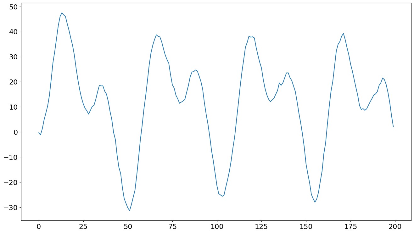
Here we simulate some data that has an weekly seasonality captured by a Fourier series.

[17]:

gen = np.random.default_rng(98765432101234567890)
idx = pd.RangeIndex(200)
det_proc = DeterministicProcess(idx, constant=True, period=52, fourier=2)
det_terms = det_proc.in_sample().to_numpy()
params = np.array([1.0, 3, -1, 4, -2])
exog = det_terms @ params
y = np.empty(200)
y[0] = det_terms[0] @ params + gen.standard_normal()
for i in range(1, 200):
    y[i] = 0.9 * y[i - 1] + det_terms[i] @ params + gen.standard_normal()
y = pd.Series(y, index=idx)
ax = y.plot()

../../../_images/examples_notebooks_generated_deterministics_28_0.png

The model is then fit using the deterministic keyword argument. seasonal defaults to False but trend defaults to "c" so this needs to be changed.

[18]:

from statsmodels.tsa.api import AutoReg

mod = AutoReg(y, 1, trend="n", deterministic=det_proc)
res = mod.fit()
print(res.summary())

                            AutoReg Model Results
==============================================================================
Dep. Variable:                      y   No. Observations:                  200
Model:                     AutoReg(1)   Log Likelihood                -270.964
Method:               Conditional MLE   S.D. of innovations              0.944
Date:                Thu, 14 Nov 2024   AIC                            555.927
Time:                        16:50:07   BIC                            578.980
Sample:                             1   HQIC                           565.258
                                  200
==============================================================================
                 coef    std err          z      P>|z|      [0.025      0.975]
------------------------------------------------------------------------------
const          0.8436      0.172      4.916      0.000       0.507       1.180
sin(1,52)      2.9738      0.160     18.587      0.000       2.660       3.287
cos(1,52)     -0.6771      0.284     -2.380      0.017      -1.235      -0.120
sin(2,52)      3.9951      0.099     40.336      0.000       3.801       4.189
cos(2,52)     -1.7206      0.264     -6.519      0.000      -2.238      -1.203
y.L1           0.9116      0.014     63.264      0.000       0.883       0.940
                                    Roots
=============================================================================
                  Real          Imaginary           Modulus         Frequency
-----------------------------------------------------------------------------
AR.1            1.0970           +0.0000j            1.0970            0.0000
-----------------------------------------------------------------------------

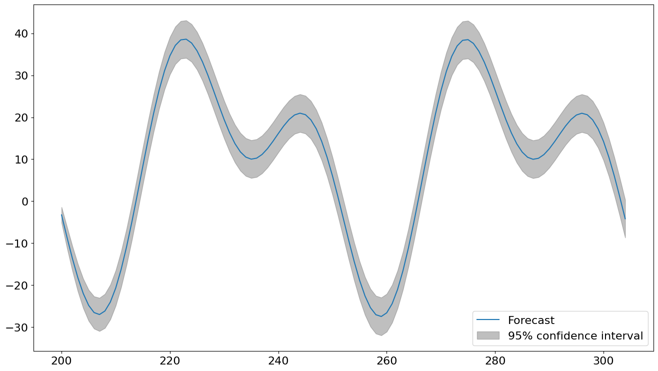
We can use the plot_predict to show the predicted values and their prediction interval. The out-of-sample deterministic values are automatically produced by the deterministic process passed to AutoReg.

[19]:

fig = res.plot_predict(200, 200 + 2 * 52, True)

../../../_images/examples_notebooks_generated_deterministics_32_0.png

[20]:

auto_reg_forecast = res.predict(200, 211)
auto_reg_forecast

[20]:

200    -3.253482
201    -8.555660
202   -13.607557
203   -18.152622
204   -21.950370
205   -24.790116
206   -26.503171
207   -26.972781
208   -26.141244
209   -24.013773
210   -20.658891
211   -16.205310
dtype: float64

Using with other models¶

Other models do not support DeterministicProcess directly. We can instead manually pass any deterministic terms as exog to model that support exogenous values.

Note that SARIMAX with exogenous variables is OLS with SARIMA errors so that the model is

\[\begin{split}\begin{align*} \nu_t & = y_t - x_t \beta \\ (1-\phi(L))\nu_t & = (1+\theta(L))\epsilon_t. \end{align*}\end{split}\]

The parameters on deterministic terms are not directly comparable to AutoReg which evolves according to the equation

\[(1-\phi(L)) y_t = x_t \beta + \epsilon_t.\]

When \(x_t\) contains only deterministic terms, these two representation are equivalent (assuming \(\theta(L)=0\) so that there is no MA).

[21]:

from statsmodels.tsa.api import SARIMAX

det_proc = DeterministicProcess(idx, period=52, fourier=2)
det_terms = det_proc.in_sample()

mod = SARIMAX(y, order=(1, 0, 0), trend="c", exog=det_terms)
res = mod.fit(disp=False)
print(res.summary())

                               SARIMAX Results
==============================================================================
Dep. Variable:                      y   No. Observations:                  200
Model:               SARIMAX(1, 0, 0)   Log Likelihood                -293.381
Date:                Thu, 14 Nov 2024   AIC                            600.763
Time:                        16:50:07   BIC                            623.851
Sample:                             0   HQIC                           610.106
                                - 200
Covariance Type:                  opg
==============================================================================
                 coef    std err          z      P>|z|      [0.025      0.975]
------------------------------------------------------------------------------
intercept      0.0796      0.140      0.567      0.571      -0.196       0.355
sin(1,52)      9.1917      0.876     10.492      0.000       7.475      10.909
cos(1,52)    -17.4351      0.891    -19.576      0.000     -19.181     -15.689
sin(2,52)      1.2509      0.466      2.683      0.007       0.337       2.165
cos(2,52)    -17.1865      0.434    -39.582      0.000     -18.038     -16.335
ar.L1          0.9957      0.007    150.751      0.000       0.983       1.009
sigma2         1.0748      0.119      9.067      0.000       0.842       1.307
===================================================================================
Ljung-Box (L1) (Q):                   2.16   Jarque-Bera (JB):                 1.03
Prob(Q):                              0.14   Prob(JB):                         0.60
Heteroskedasticity (H):               0.71   Skew:                            -0.14
Prob(H) (two-sided):                  0.16   Kurtosis:                         2.78
===================================================================================

Warnings:
[1] Covariance matrix calculated using the outer product of gradients (complex-step).

The forecasts are similar but differ since the parameters of the SARIMAX are estimated using MLE while AutoReg uses OLS.

[22]:

sarimax_forecast = res.forecast(12, exog=det_proc.out_of_sample(12))
df = pd.concat([auto_reg_forecast, sarimax_forecast], axis=1)
df.columns = columns = ["AutoReg", "SARIMAX"]
df

[22]:

	AutoReg	SARIMAX
200	-3.253482	-2.956589
201	-8.555660	-7.985653
202	-13.607557	-12.794185
203	-18.152622	-17.131131
204	-21.950370	-20.760701
205	-24.790116	-23.475800
206	-26.503171	-25.109977
207	-26.972781	-25.547191
208	-26.141244	-24.728829
209	-24.013773	-22.657570
210	-20.658891	-19.397843
211	-16.205310	-15.072875

Last update: Nov 14, 2024