

Regression diagnostics#
This example file shows how to use a few of the statsmodels regression diagnostic tests in a real-life context. You can learn about more tests and find out more information about the tests here on the Regression Diagnostics page.
Note that most of the tests described here only return a tuple of numbers, without any annotation. A full description of outputs is always included in the docstring and in the online statsmodels documentation. For presentation purposes, we use the zip(name,test) construct to pretty-print short descriptions in the examples below.
Estimate a regression model#
[1]:
%matplotlib inline
[2]:
import matplotlib.pyplot as plt
import numpy as np
import pandas as pd

import statsmodels.formula.api as smf
import statsmodels.stats.api as sms


# Helper function
def display(name, test):
    for lbl, val in zip(name, test, strict=True):
        if val is None:
            continue
        out = val if isinstance(val, str) else float(val)
        print(f"{lbl}: {out}")


# Load data
url = "https://raw.githubusercontent.com/vincentarelbundock/Rdatasets/master/csv/HistData/Guerry.csv"
dat = pd.read_csv(url)

# Fit regression model (using the natural log of one of the regressors)
results = smf.ols("Lottery ~ Literacy + np.log(Pop1831)", data=dat).fit()

# Inspect the results
print(results.summary())
                            OLS Regression Results
==============================================================================
Dep. Variable:                Lottery   R-squared:                       0.348
Model:                            OLS   Adj. R-squared:                  0.333
Method:                 Least Squares   F-statistic:                     22.20
Date:                Wed, 09 Sep 2026   Prob (F-statistic):           1.90e-08
Time:                        05:40:12   Log-Likelihood:                -379.82
No. Observations:                  86   AIC:                             765.6
Df Residuals:                      83   BIC:                             773.0
Df Model:                           2
Covariance Type:            nonrobust
===================================================================================
                      coef    std err          t      P>|t|      [0.025      0.975]
-----------------------------------------------------------------------------------
Intercept         246.4341     35.233      6.995      0.000     176.358     316.510
Literacy           -0.4889      0.128     -3.832      0.000      -0.743      -0.235
np.log(Pop1831)   -31.3114      5.977     -5.239      0.000     -43.199     -19.424
==============================================================================
Omnibus:                        3.713   Durbin-Watson:                   2.019
Prob(Omnibus):                  0.156   Jarque-Bera (JB):                3.394
Skew:                          -0.487   Prob(JB):                        0.183
Kurtosis:                       3.003   Cond. No.                         702.
==============================================================================

Notes:
[1] Standard Errors assume that the covariance matrix of the errors is correctly specified.
Normality of the residuals#
Omni test:
[3]:
name = ["Chi^2", "Two-tail probability"]
test = sms.omni_normtest(results.resid)
display(name, test)
Chi^2: 3.7134378115972093
Two-tail probability: 0.15618424580304607
Jarque-Bera test:
Kurtosis below is the sample kurtosis, not the excess kurtosis. A sample from the normal distribution has kurtosis equal to 3.
[4]:
name = ["Jarque-Bera test", "Chi^2 two-tail prob.", "Skew", "Kurtosis"]
test = sms.jarque_bera(results.resid)
display(name, test)
Jarque-Bera test: 3.3936080248431884
Chi^2 two-tail prob.: 0.18326831231663174
Skew: -0.4865803431122353
Kurtosis: 3.0034177578816363
Autorelation#
Durbin-Watson test:
DW statistic always ranges from 0 to 4. The closer to 2, the less autocorrelation is in the sample.
[5]:
name = ["Durbin-Watson statistic"]
test = [sms.durbin_watson(results.resid)]
display(name, test)
Durbin-Watson statistic: 2.019216822454508
Breusch–Godfrey test for serial correlation:
[6]:
name = [
    "Breusch-Pagan Lagrange multiplier test statistic",
    "p-value",
    "f-value",
    "f p-value",
    "store",
]
test = sms.acorr_breusch_godfrey(results, result_object=True)
display(name, test)
Breusch-Pagan Lagrange multiplier test statistic: 2.9930462802518636
p-value: 0.9815872336580146
f-value: 0.26322177681170067
f p-value: 0.9871702599878219
Multicollinearity#
Condition number
[7]:
name = ["Condition Number"]
test = [np.linalg.cond(results.model.exog)]
display(name, test)
Condition Number: 702.1792145490066
Influence tests#
Once created, an object of class OLSInfluence holds attributes and methods that allow users to assess the influence of each observation. For example, we can compute and extract the first few rows of DFbetas by:
[8]:
from statsmodels.stats.outliers_influence import OLSInfluence

test_class = OLSInfluence(results)
test_class.dfbetas[:5, :]
[8]:
array([[-0.00301154,  0.00290872,  0.00118179],
       [-0.06425662,  0.04043093,  0.06281609],
       [ 0.01554894, -0.03556038, -0.00905336],
       [ 0.17899858,  0.04098207, -0.18062352],
       [ 0.29679073,  0.21249207, -0.3213655 ]])
Explore other options by typing dir(influence_test)
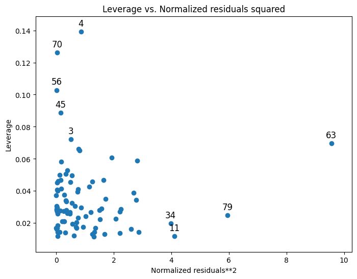
Useful information on leverage can also be plotted:
[9]:
from statsmodels.graphics.regressionplots import plot_leverage_resid2

fig, ax = plt.subplots(figsize=(8, 6))
fig = plot_leverage_resid2(results, ax=ax)
Other plotting options can be found on the Graphics page.
Heteroskedasticity tests#
Breush-Pagan test:
[10]:
name = ["Lagrange multiplier statistic", "p-value", "f-value", "f p-value"]
test = sms.het_breuschpagan(results.resid, results.model.exog)
display(name, test)
Lagrange multiplier statistic: 4.893213374094043
p-value: 0.0865869050235184
f-value: 2.5037159462564804
f p-value: 0.08794028782672657
Goldfeld-Quandt test
[11]:
name = ["F statistic", "p-value", "ordering", "store"]
# result_object=True for changes coming later
test = sms.het_goldfeldquandt(results.resid, results.model.exog, result_object=True)
display(name, test)
F statistic: 1.1002422436378148
p-value: 0.3820295068692514
ordering: increasing
Linearity#
Harvey-Collier multiplier test for Null hypothesis that the linear specification is correct:
[12]:
name = ["t value", "p value"]
test = sms.linear_harvey_collier(results)
display(name, test)
t value: -1.0796490077759802
p value: 0.28346392475692195