statsmodels.tsa.filters.hp_filter.hpfilter¶

statsmodels.tsa.filters.hp_filter.hpfilter(x, lamb=1600)[source]¶

Hodrick-Prescott filter.

Parameters:¶

xarray_like

The time series to filter, 1-d.

lambfloat

The Hodrick-Prescott smoothing parameter. A value of 1600 is suggested for quarterly data. Ravn and Uhlig suggest using a value of 6.25 (1600/4**4) for annual data and 129600 (1600*3**4) for monthly data.

Returns:¶

cyclendarray

The estimated cycle in the data given lamb.

trendndarray

The estimated trend in the data given lamb.

See also

statsmodels.tsa.filters.bk_filter.bkfilter

Baxter-King filter.

statsmodels.tsa.filters.cf_filter.cffilter

The Christiano Fitzgerald asymmetric, random walk filter.

statsmodels.tsa.seasonal.seasonal_decompose

Decompose a time series using moving averages.

statsmodels.tsa.seasonal.STL

Season-Trend decomposition using LOESS.

Notes

The HP filter removes a smooth trend, T, from the data x. by solving

min sum((x[t] - T[t])**2 + lamb*((T[t+1] - T[t]) - (T[t] - T[t-1]))**2)

T t

Here we implemented the HP filter as a ridge-regression rule using scipy.sparse. In this sense, the solution can be written as

T = inv(I + lamb*K’K)x

where I is a nobs x nobs identity matrix, and K is a (nobs-2) x nobs matrix such that

K[i,j] = 1 if i == j or i == j + 2 K[i,j] = -2 if i == j + 1 K[i,j] = 0 otherwise

See the notebook Time Series Filters for an overview.

References

Hodrick, R.J, and E. C. Prescott. 1980. “Postwar U.S. Business Cycles: An

Empirical Investigation.” Carnegie Mellon University discussion paper no. 451.

Ravn, M.O and H. Uhlig. 2002. “Notes On Adjusted the Hodrick-Prescott

Filter for the Frequency of Observations.” The Review of Economics and Statistics, 84(2), 371-80.

Examples

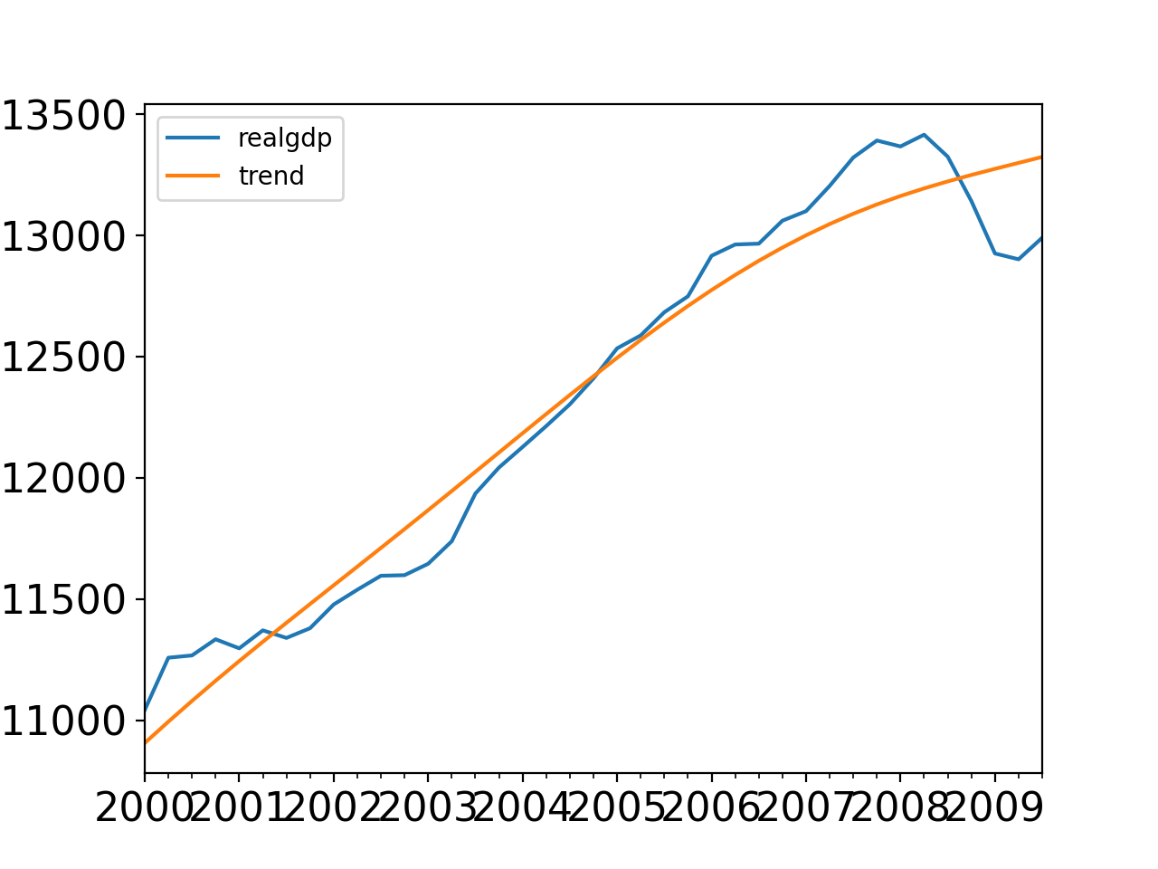
>>> import statsmodels.api as sm
>>> import pandas as pd
>>> dta = sm.datasets.macrodata.load_pandas().data
>>> index = pd.period_range('1959Q1', '2009Q3', freq='Q')
>>> dta.set_index(index, inplace=True)

>>> cycle, trend = sm.tsa.filters.hpfilter(dta.realgdp, 1600)
>>> gdp_decomp = dta[['realgdp']]
>>> gdp_decomp["cycle"] = cycle
>>> gdp_decomp["trend"] = trend

>>> import matplotlib.pyplot as plt
>>> fig, ax = plt.subplots()
>>> gdp_decomp[["realgdp", "trend"]]["2000-03-31":].plot(ax=ax,
...                                                      fontsize=16)
>>> plt.show()

(Source code, png, hires.png, pdf)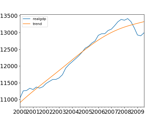