statsmodels.tsa.seasonal.MSTL¶

class statsmodels.tsa.seasonal.MSTL(endog, periods=None, windows=None, lmbda=None, iterate=2, stl_kwargs=None)[source]¶

Season-Trend decomposition using LOESS for multiple seasonalities.

Added in version 0.14.0.

Parameters:¶

endogarray_like

Data to be decomposed. Must be squeezable to 1-d.

periods{int, array_like, None}, optional

Periodicity of the seasonal components. If None and endog is a pandas Series or DataFrame, attempts to determine from endog. If endog is a ndarray, periods must be provided.

windows{int, array_like, None}, optional

Length of the seasonal smoothers for each corresponding period. Must be an odd integer, and should normally be >= 7 (default). If None then default values determined using 7 + 4 * np.arange(1, n + 1, 1) where n is number of seasonal components.

lmbda{float, str, None}, optional

The lambda parameter for the Box-Cox transform to be applied to endog prior to decomposition. If None, no transform is applied. If “auto”, a value will be estimated that maximizes the log-likelihood function.

iterateint, optional

Number of iterations to use to refine the seasonal component.

stl_kwargs: dict, optional

Arguments to pass to STL.

See also

statsmodels.tsa.seasonal.STL

References

[1]

K. Bandura, R.J. Hyndman, and C. Bergmeir (2021) MSTL: A Seasonal-Trend Decomposition Algorithm for Time Series with Multiple Seasonal Patterns. arXiv preprint arXiv:2107.13462.

Examples

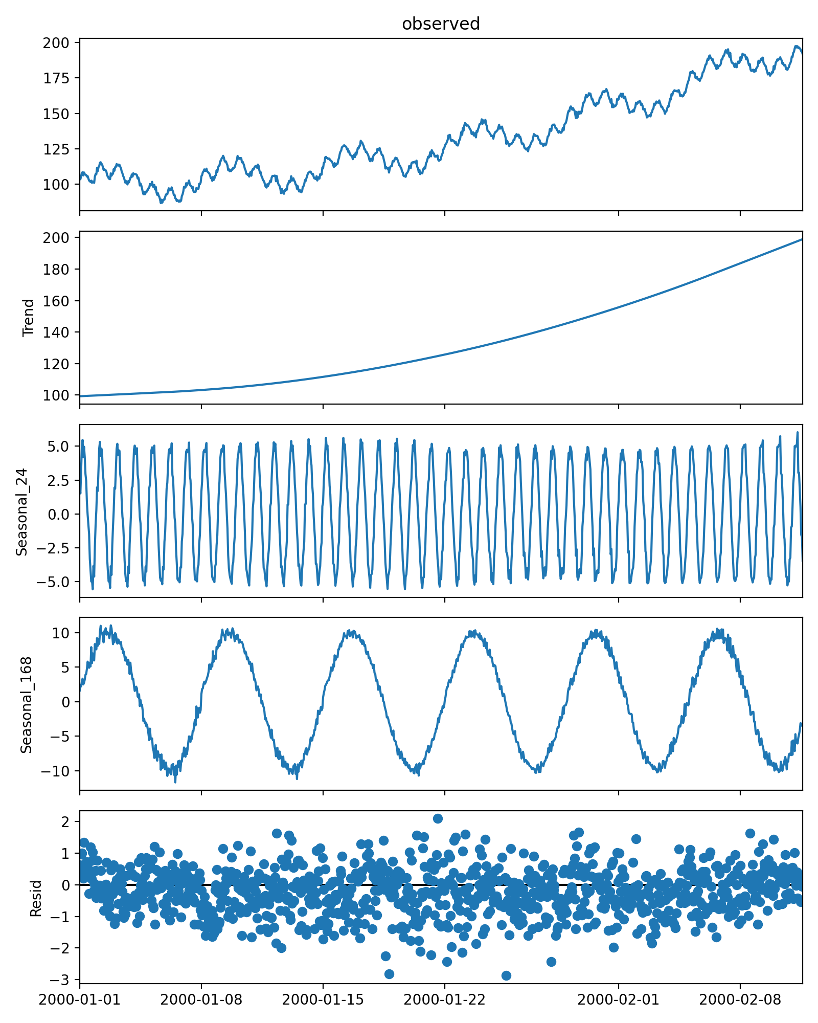
Start by creating a toy dataset with hourly frequency and multiple seasonal components.

>>> import numpy as np
>>> import matplotlib.pyplot as plt
>>> import pandas as pd
>>> pd.plotting.register_matplotlib_converters()
>>> np.random.seed(0)
>>> t = np.arange(1, 1000)
>>> trend = 0.0001 * t ** 2 + 100
>>> daily_seasonality = 5 * np.sin(2 * np.pi * t / 24)
>>> weekly_seasonality = 10 * np.sin(2 * np.pi * t / (24 * 7))
>>> noise = np.random.randn(len(t))
>>> y = trend + daily_seasonality + weekly_seasonality + noise
>>> index = pd.date_range(start='2000-01-01', periods=len(t), freq='H')
>>> data = pd.DataFrame(data=y, index=index)

Use MSTL to decompose the time series into two seasonal components with periods 24 (daily seasonality) and 24*7 (weekly seasonality).

>>> from statsmodels.tsa.seasonal import MSTL
>>> res = MSTL(data, periods=(24, 24*7)).fit()
>>> res.plot()
>>> plt.tight_layout()
>>> plt.show()

(Source code, png, hires.png, pdf)

Methods

fit()

Estimate a trend component, multiple seasonal components, and a residual component.