Kernel Density Estimation¶

Kernel density estimation is the process of estimating an unknown probability density function using a kernel function \(K(u)\). While a histogram counts the number of data points in somewhat arbitrary regions, a kernel density estimate is a function defined as the sum of a kernel function on every data point. The kernel function typically exhibits the following properties:

Symmetry such that \(K(u) = K(-u)\).
Normalization such that \(\int_{-\infty}^{\infty} K(u) \ du = 1\) .
Monotonically decreasing such that \(K'(u) < 0\) when \(u > 0\).
Expected value equal to zero such that \(\mathrm{E}[K] = 0\).

For more information about kernel density estimation, see for instance Wikipedia - Kernel density estimation.

A univariate kernel density estimator is implemented in sm.nonparametric.KDEUnivariate. In this example we will show the following:

Basic usage, how to fit the estimator.
The effect of varying the bandwidth of the kernel using the bw argument.
The various kernel functions available using the kernel argument.

[1]:

%matplotlib inline
import numpy as np
from scipy import stats
import statsmodels.api as sm
import matplotlib.pyplot as plt
from statsmodels.distributions.mixture_rvs import mixture_rvs

A univariate example¶

[2]:

np.random.seed(12345)  # Seed the random number generator for reproducible results

We create a bimodal distribution: a mixture of two normal distributions with locations at -1 and 1.

[3]:

# Location, scale and weight for the two distributions
dist1_loc, dist1_scale, weight1 = -1, 0.5, 0.25
dist2_loc, dist2_scale, weight2 = 1, 0.5, 0.75

# Sample from a mixture of distributions
obs_dist = mixture_rvs(
    prob=[weight1, weight2],
    size=250,
    dist=[stats.norm, stats.norm],
    kwargs=(
        dict(loc=dist1_loc, scale=dist1_scale),
        dict(loc=dist2_loc, scale=dist2_scale),
    ),
)

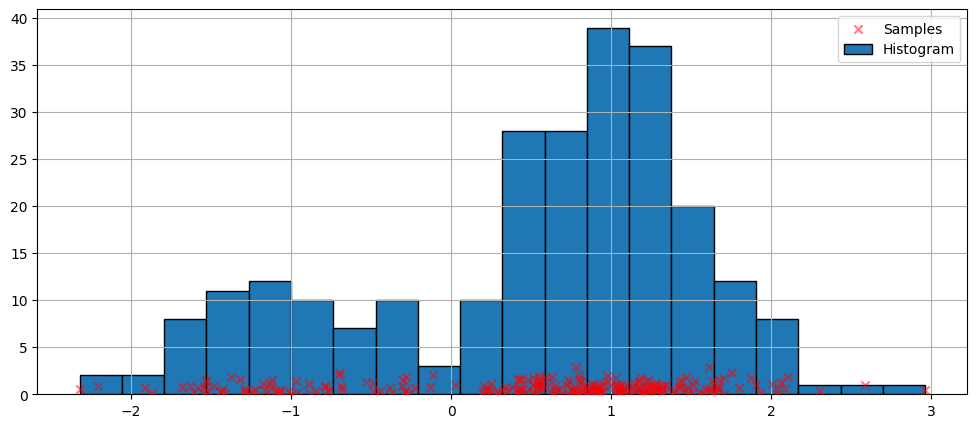
The simplest non-parametric technique for density estimation is the histogram.

[4]:

fig = plt.figure(figsize=(12, 5))
ax = fig.add_subplot(111)

# Scatter plot of data samples and histogram
ax.scatter(
    obs_dist,
    np.abs(np.random.randn(obs_dist.size)),
    zorder=15,
    color="red",
    marker="x",
    alpha=0.5,
    label="Samples",
)
lines = ax.hist(obs_dist, bins=20, edgecolor="k", label="Histogram")

ax.legend(loc="best")
ax.grid(True, zorder=-5)

../../../_images/examples_notebooks_generated_kernel_density_7_0.png

Fitting with the default arguments¶

The histogram above is discontinuous. To compute a continuous probability density function, we can use kernel density estimation.

We initialize a univariate kernel density estimator using KDEUnivariate.

[5]:

kde = sm.nonparametric.KDEUnivariate(obs_dist)
kde.fit()  # Estimate the densities

[5]:

<statsmodels.nonparametric.kde.KDEUnivariate at 0x7fed558239a0>

We present a figure of the fit, as well as the true distribution.

[6]:

fig = plt.figure(figsize=(12, 5))
ax = fig.add_subplot(111)

# Plot the histogram
ax.hist(
    obs_dist,
    bins=20,
    density=True,
    label="Histogram from samples",
    zorder=5,
    edgecolor="k",
    alpha=0.5,
)

# Plot the KDE as fitted using the default arguments
ax.plot(kde.support, kde.density, lw=3, label="KDE from samples", zorder=10)

# Plot the true distribution
true_values = (
    stats.norm.pdf(loc=dist1_loc, scale=dist1_scale, x=kde.support) * weight1
    + stats.norm.pdf(loc=dist2_loc, scale=dist2_scale, x=kde.support) * weight2
)
ax.plot(kde.support, true_values, lw=3, label="True distribution", zorder=15)

# Plot the samples
ax.scatter(
    obs_dist,
    np.abs(np.random.randn(obs_dist.size)) / 40,
    marker="x",
    color="red",
    zorder=20,
    label="Samples",
    alpha=0.5,
)

ax.legend(loc="best")
ax.grid(True, zorder=-5)

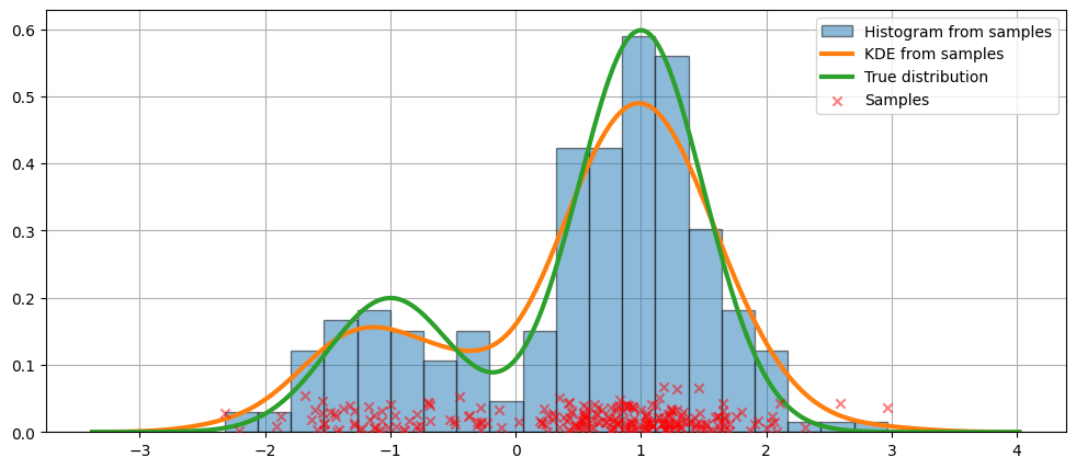
../../../_images/examples_notebooks_generated_kernel_density_12_0.png

In the code above, default arguments were used. We can also vary the bandwidth of the kernel, as we will now see.

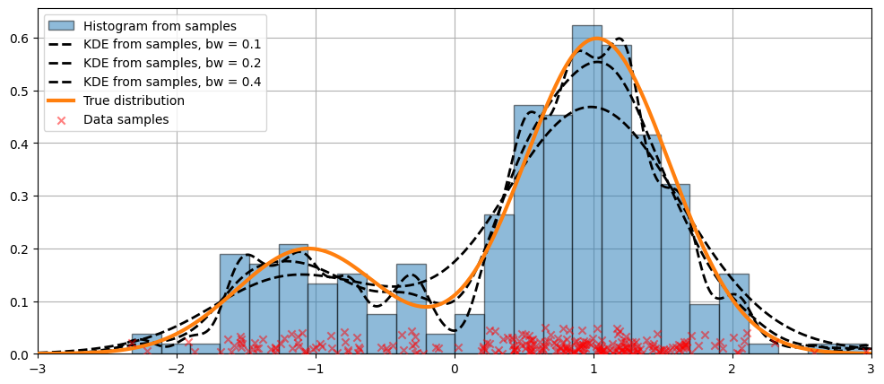
Varying the bandwidth using the `bw` argument¶

The bandwidth of the kernel can be adjusted using the bw argument. In the following example, a bandwidth of bw=0.2 seems to fit the data well.

[7]:

fig = plt.figure(figsize=(12, 5))
ax = fig.add_subplot(111)

# Plot the histogram
ax.hist(
    obs_dist,
    bins=25,
    label="Histogram from samples",
    zorder=5,
    edgecolor="k",
    density=True,
    alpha=0.5,
)

# Plot the KDE for various bandwidths
for bandwidth in [0.1, 0.2, 0.4]:
    kde.fit(bw=bandwidth)  # Estimate the densities
    ax.plot(
        kde.support,
        kde.density,
        "--",
        lw=2,
        color="k",
        zorder=10,
        label="KDE from samples, bw = {}".format(round(bandwidth, 2)),
    )

# Plot the true distribution
ax.plot(kde.support, true_values, lw=3, label="True distribution", zorder=15)

# Plot the samples
ax.scatter(
    obs_dist,
    np.abs(np.random.randn(obs_dist.size)) / 50,
    marker="x",
    color="red",
    zorder=20,
    label="Data samples",
    alpha=0.5,
)

ax.legend(loc="best")
ax.set_xlim([-3, 3])
ax.grid(True, zorder=-5)

../../../_images/examples_notebooks_generated_kernel_density_16_0.png

Comparing kernel functions¶

In the example above, a Gaussian kernel was used. Several other kernels are also available.

[8]:

from statsmodels.nonparametric.kde import kernel_switch

list(kernel_switch.keys())

[8]:

['gau', 'epa', 'uni', 'tri', 'biw', 'triw', 'cos', 'cos2', 'tric']

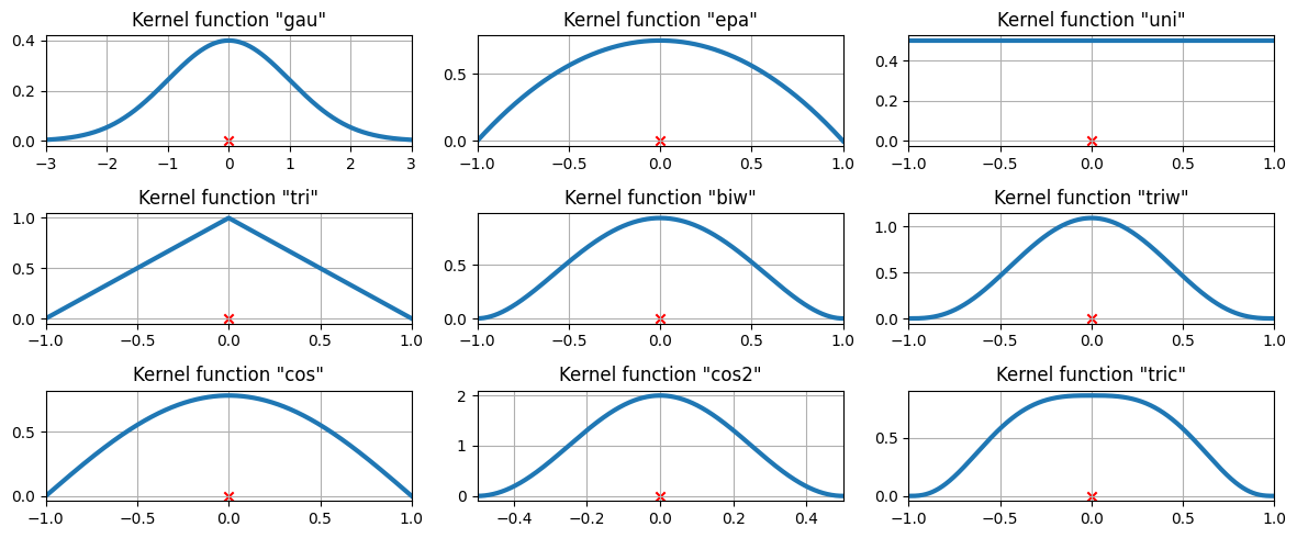
The available kernel functions¶

[9]:

# Create a figure
fig = plt.figure(figsize=(12, 5))

# Enumerate every option for the kernel
for i, (ker_name, ker_class) in enumerate(kernel_switch.items()):

    # Initialize the kernel object
    kernel = ker_class()

    # Sample from the domain
    domain = kernel.domain or [-3, 3]
    x_vals = np.linspace(*domain, num=2 ** 10)
    y_vals = kernel(x_vals)

    # Create a subplot, set the title
    ax = fig.add_subplot(3, 3, i + 1)
    ax.set_title('Kernel function "{}"'.format(ker_name))
    ax.plot(x_vals, y_vals, lw=3, label="{}".format(ker_name))
    ax.scatter([0], [0], marker="x", color="red")
    plt.grid(True, zorder=-5)
    ax.set_xlim(domain)

plt.tight_layout()

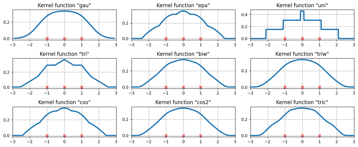
../../../_images/examples_notebooks_generated_kernel_density_21_0.png

The available kernel functions on three data points¶

We now examine how the kernel density estimate will fit to three equally spaced data points.

[10]:

# Create three equidistant points
data = np.linspace(-1, 1, 3)
kde = sm.nonparametric.KDEUnivariate(data)

# Create a figure
fig = plt.figure(figsize=(12, 5))

# Enumerate every option for the kernel
for i, kernel in enumerate(kernel_switch.keys()):

    # Create a subplot, set the title
    ax = fig.add_subplot(3, 3, i + 1)
    ax.set_title('Kernel function "{}"'.format(kernel))

    # Fit the model (estimate densities)
    kde.fit(kernel=kernel, fft=False, gridsize=2 ** 10)

    # Create the plot
    ax.plot(kde.support, kde.density, lw=3, label="KDE from samples", zorder=10)
    ax.scatter(data, np.zeros_like(data), marker="x", color="red")
    plt.grid(True, zorder=-5)
    ax.set_xlim([-3, 3])

plt.tight_layout()

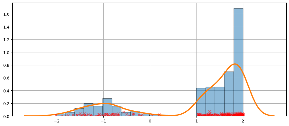
../../../_images/examples_notebooks_generated_kernel_density_24_0.png

A more difficult case¶

The fit is not always perfect. See the example below for a harder case.

[11]:

obs_dist = mixture_rvs(
    [0.25, 0.75],
    size=250,
    dist=[stats.norm, stats.beta],
    kwargs=(dict(loc=-1, scale=0.5), dict(loc=1, scale=1, args=(1, 0.5))),
)

[12]:

kde = sm.nonparametric.KDEUnivariate(obs_dist)
kde.fit()

[12]:

<statsmodels.nonparametric.kde.KDEUnivariate at 0x7fed52347940>

[13]:

fig = plt.figure(figsize=(12, 5))
ax = fig.add_subplot(111)
ax.hist(obs_dist, bins=20, density=True, edgecolor="k", zorder=4, alpha=0.5)
ax.plot(kde.support, kde.density, lw=3, zorder=7)
# Plot the samples
ax.scatter(
    obs_dist,
    np.abs(np.random.randn(obs_dist.size)) / 50,
    marker="x",
    color="red",
    zorder=20,
    label="Data samples",
    alpha=0.5,
)
ax.grid(True, zorder=-5)

../../../_images/examples_notebooks_generated_kernel_density_28_0.png

The KDE is a distribution¶

Since the KDE is a distribution, we can access attributes and methods such as:

entropy
evaluate
cdf
icdf
sf
cumhazard

[14]:

obs_dist = mixture_rvs(
    [0.25, 0.75],
    size=1000,
    dist=[stats.norm, stats.norm],
    kwargs=(dict(loc=-1, scale=0.5), dict(loc=1, scale=0.5)),
)
kde = sm.nonparametric.KDEUnivariate(obs_dist)
kde.fit(gridsize=2 ** 10)

[14]:

<statsmodels.nonparametric.kde.KDEUnivariate at 0x7fed535c1c00>

[15]:

kde.entropy

[15]:

1.314324140492138

[16]:

kde.evaluate(-1)

[16]:

array([0.18085886])

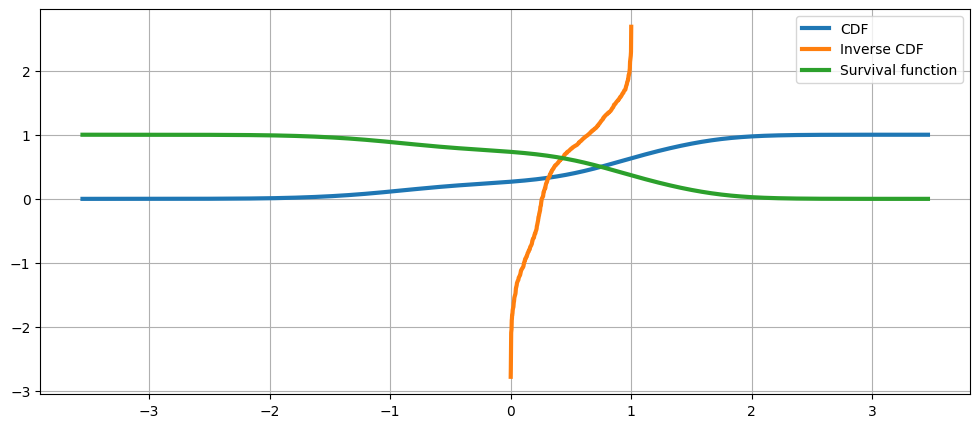
Cumulative distribution, it’s inverse, and the survival function¶

[17]:

fig = plt.figure(figsize=(12, 5))
ax = fig.add_subplot(111)

ax.plot(kde.support, kde.cdf, lw=3, label="CDF")
ax.plot(np.linspace(0, 1, num=kde.icdf.size), kde.icdf, lw=3, label="Inverse CDF")
ax.plot(kde.support, kde.sf, lw=3, label="Survival function")
ax.legend(loc="best")
ax.grid(True, zorder=-5)

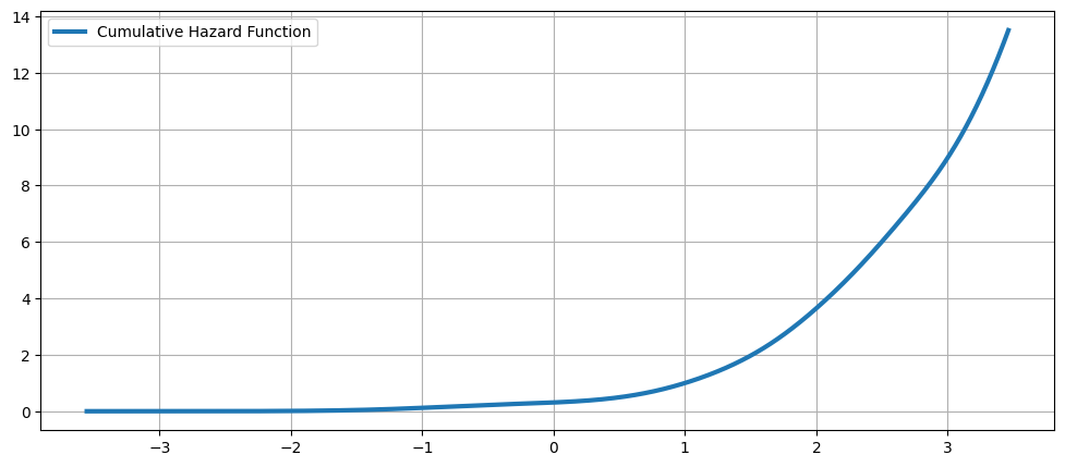
../../../_images/examples_notebooks_generated_kernel_density_34_0.png

The Cumulative Hazard Function¶

[18]:

fig = plt.figure(figsize=(12, 5))
ax = fig.add_subplot(111)
ax.plot(kde.support, kde.cumhazard, lw=3, label="Cumulative Hazard Function")
ax.legend(loc="best")
ax.grid(True, zorder=-5)

../../../_images/examples_notebooks_generated_kernel_density_36_0.png

Last update: Oct 03, 2024