Prediction (out of sample)
[1]:
%matplotlib inline
[2]:
import numpy as np
import matplotlib.pyplot as plt

import statsmodels.api as sm

plt.rc("figure", figsize=(16, 8))
plt.rc("font", size=14)
Artificial data
[3]:
nsample = 50
sig = 0.25
x1 = np.linspace(0, 20, nsample)
X = np.column_stack((x1, np.sin(x1), (x1 - 5) ** 2))
X = sm.add_constant(X)
beta = [5.0, 0.5, 0.5, -0.02]
y_true = np.dot(X, beta)
y = y_true + sig * np.random.normal(size=nsample)
Estimation
[4]:
olsmod = sm.OLS(y, X)
olsres = olsmod.fit()
print(olsres.summary())
                            OLS Regression Results
==============================================================================
Dep. Variable:                      y   R-squared:                       0.974
Model:                            OLS   Adj. R-squared:                  0.973
Method:                 Least Squares   F-statistic:                     584.3
Date:                Sun, 14 Jun 2026   Prob (F-statistic):           1.30e-36
Time:                        22:50:29   Log-Likelihood:                -9.6142
No. Observations:                  50   AIC:                             27.23
Df Residuals:                      46   BIC:                             34.88
Df Model:                           3
Covariance Type:            nonrobust
==============================================================================
                 coef    std err          t      P>|t|      [0.025      0.975]
------------------------------------------------------------------------------
const          5.1365      0.104     49.288      0.000       4.927       5.346
x1             0.4800      0.016     29.866      0.000       0.448       0.512
x2             0.4726      0.063      7.480      0.000       0.345       0.600
x3            -0.0183      0.001    -12.987      0.000      -0.021      -0.015
==============================================================================
Omnibus:                        1.362   Durbin-Watson:                   2.139
Prob(Omnibus):                  0.506   Jarque-Bera (JB):                0.602
Skew:                          -0.023   Prob(JB):                        0.740
Kurtosis:                       3.536   Cond. No.                         221.
==============================================================================

Notes:
[1] Standard Errors assume that the covariance matrix of the errors is correctly specified.
In-sample prediction
[5]:
ypred = olsres.predict(X)
print(ypred)
[ 4.67834355  5.13360472  5.55193985  5.90759305  6.18410359  6.37701037
  6.49458484  6.55647205  6.59046299  6.62792867  6.69866587  6.82600168
  7.02296089  7.29012608  7.61554187  7.97667919  8.3441367   8.68647141
  8.97536461  9.1902746   9.32181158  9.37328045  9.36013774  9.3074522
  9.24578605  9.20617369  9.21502288  9.28977596  9.43604415  9.64668566
  9.90297902 10.17769903 10.43958971 10.65849962 10.81033565 10.88102143
 10.86881005 10.78457107 10.65000469 10.49407645 10.3482583  10.24135783
 10.19478525 10.21903579 10.31196535 10.45914273 10.63622071 10.81293617
 10.95808224 11.04463553]
Create a new sample of explanatory variables Xnew, predict and plot
[6]:
x1n = np.linspace(20.5, 25, 10)
Xnew = np.column_stack((x1n, np.sin(x1n), (x1n - 5) ** 2))
Xnew = sm.add_constant(Xnew)
ynewpred = olsres.predict(Xnew)  # predict out of sample
print(ynewpred)
[11.04479349 10.92044734 10.69013038 10.39607768 10.09388542  9.83889903
  9.67266271  9.61274795  9.6484514   9.74341546]
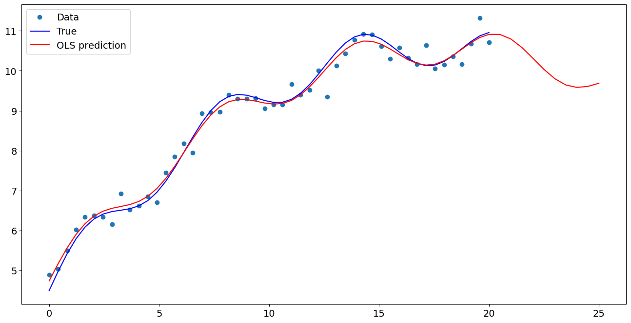
Plot comparison
[7]:
import matplotlib.pyplot as plt

fig, ax = plt.subplots()
ax.plot(x1, y, "o", label="Data")
ax.plot(x1, y_true, "b-", label="True")
ax.plot(np.hstack((x1, x1n)), np.hstack((ypred, ynewpred)), "r", label="OLS prediction")
ax.legend(loc="best")
[7]:
<matplotlib.legend.Legend at 0x7f58d86400a0>
Predicting with Formulas
Using formulas can make both estimation and prediction a lot easier
[8]:
from statsmodels.formula.api import ols

data = {"x1": x1, "y": y}

res = ols("y ~ x1 + np.sin(x1) + I((x1-5)**2)", data=data).fit()
We use the I to indicate use of the Identity transform. Ie., we do not want any expansion magic from using **2
[9]:
res.params
[9]:
Intercept           5.136530
x1                  0.480016
np.sin(x1)          0.472593
I((x1 - 5) ** 2)   -0.018327
dtype: float64
Now we only have to pass the single variable and we get the transformed right-hand side variables automatically
[10]:
res.predict(exog=dict(x1=x1n))
[10]:
0    11.044793
1    10.920447
2    10.690130
3    10.396078
4    10.093885
5     9.838899
6     9.672663
7     9.612748
8     9.648451
9     9.743415
dtype: float64