VARMAX models
This is a brief introduction notebook to VARMAX models in statsmodels. The VARMAX model is generically specified as:
where \(y_t\) is a \(\mathrm{k_endog} \times 1\) vector.
[1]:
%matplotlib inline
[2]:
import matplotlib.pyplot as plt
import numpy as np
import pandas as pd
import statsmodels.api as sm
[3]:
import shutil

import requests


def download_file(url):
    local_filename = url.split("/")[-1]
    with requests.get(url, stream=True) as r:
        with open(local_filename, "wb") as f:
            shutil.copyfileobj(r.raw, f)

    return local_filename


filename = download_file("https://www.stata-press.com/data/r12/lutkepohl2.dta")

dta = pd.read_stata(filename)
dta.index = dta.qtr
dta.index.freq = dta.index.inferred_freq
endog = dta.loc["1960-04-01":"1978-10-01", ["dln_inv", "dln_inc", "dln_consump"]]
Model specification
The VARMAX class in statsmodels allows estimation of VAR, VMA, and VARMA models (through the order argument), optionally with a constant term (via the trend argument). Exogenous regressors may also be included (as usual in statsmodels, by the exog argument), and in this way a time trend may be added. Finally, the class allows measurement error (via the measurement_error argument) and allows specifying either a diagonal or unstructured innovation covariance matrix (via the
error_cov_type argument).
Example 1: VAR
Below is a simple VARX(2) model in two endogenous variables and an exogenous series, but no constant term. Notice that we needed to allow for more iterations than the default (which is maxiter=50) in order for the likelihood estimation to converge. This is not unusual in VAR models which have to estimate a large number of parameters, often on a relatively small number of time series: this model, for example, estimates 27 parameters off of 75 observations of 3 variables.
[4]:
exog = endog["dln_consump"]
mod = sm.tsa.VARMAX(endog[["dln_inv", "dln_inc"]], order=(2, 0), trend="n", exog=exog)
res = mod.fit(maxiter=1000, disp=False)
print(res.summary())
                             Statespace Model Results
==================================================================================
Dep. Variable:     ['dln_inv', 'dln_inc']   No. Observations:                   75
Model:                            VARX(2)   Log Likelihood                 361.032
Date:                    Sun, 14 Jun 2026   AIC                           -696.063
Time:                            23:03:56   BIC                           -665.936
Sample:                        04-01-1960   HQIC                          -684.033
                             - 10-01-1978
Covariance Type:                      opg
===================================================================================
Ljung-Box (L1) (Q):            0.03, 10.27   Jarque-Bera (JB):          10.97, 2.38
Prob(Q):                        0.86, 0.00   Prob(JB):                   0.00, 0.30
Heteroskedasticity (H):         0.45, 0.40   Skew:                      0.15, -0.38
Prob(H) (two-sided):            0.05, 0.02   Kurtosis:                   4.85, 3.44
                            Results for equation dln_inv
====================================================================================
                       coef    std err          z      P>|z|      [0.025      0.975]
------------------------------------------------------------------------------------
L1.dln_inv          -0.2454      0.092     -2.654      0.008      -0.427      -0.064
L1.dln_inc           0.2859      0.448      0.638      0.524      -0.593       1.165
L2.dln_inv          -0.1629      0.155     -1.052      0.293      -0.466       0.141
L2.dln_inc           0.0893      0.422      0.212      0.832      -0.737       0.916
beta.dln_consump     0.9504      0.639      1.488      0.137      -0.302       2.203
                            Results for equation dln_inc
====================================================================================
                       coef    std err          z      P>|z|      [0.025      0.975]
------------------------------------------------------------------------------------
L1.dln_inv           0.0618      0.036      1.715      0.086      -0.009       0.132
L1.dln_inc           0.0851      0.107      0.793      0.428      -0.125       0.296
L2.dln_inv           0.0077      0.033      0.235      0.814      -0.057       0.072
L2.dln_inc           0.0358      0.134      0.267      0.790      -0.227       0.299
beta.dln_consump     0.7722      0.112      6.885      0.000       0.552       0.992
                                  Error covariance matrix
============================================================================================
                               coef    std err          z      P>|z|      [0.025      0.975]
--------------------------------------------------------------------------------------------
sqrt.var.dln_inv             0.0433      0.004     12.310      0.000       0.036       0.050
sqrt.cov.dln_inv.dln_inc  8.489e-06      0.002      0.004      0.997      -0.004       0.004
sqrt.var.dln_inc             0.0109      0.001     11.202      0.000       0.009       0.013
============================================================================================

Warnings:
[1] Covariance matrix calculated using the outer product of gradients (complex-step).
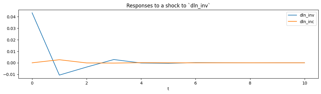
From the estimated VAR model, we can plot the impulse response functions of the endogenous variables.
[5]:
ax = res.impulse_responses(10, orthogonalized=True, impulse=[1, 0]).plot(
    figsize=(13, 3)
)
ax.set(xlabel="t", title="Responses to a shock to `dln_inv`");
Example 2: VMA
A vector moving average model can also be formulated. Below we show a VMA(2) on the same data, but where the innovations to the process are uncorrelated. In this example we leave out the exogenous regressor but now include the constant term.
[6]:
mod = sm.tsa.VARMAX(
    endog[["dln_inv", "dln_inc"]], order=(0, 2), error_cov_type="diagonal"
)
res = mod.fit(maxiter=1000, disp=False)
print(res.summary())
                             Statespace Model Results
==================================================================================
Dep. Variable:     ['dln_inv', 'dln_inc']   No. Observations:                   75
Model:                             VMA(2)   Log Likelihood                 353.880
                              + intercept   AIC                           -683.761
Date:                    Sun, 14 Jun 2026   BIC                           -655.951
Time:                            23:03:58   HQIC                          -672.656
Sample:                        04-01-1960
                             - 10-01-1978
Covariance Type:                      opg
===================================================================================
Ljung-Box (L1) (Q):             0.00, 0.04   Jarque-Bera (JB):         13.44, 14.28
Prob(Q):                        1.00, 0.84   Prob(JB):                   0.00, 0.00
Heteroskedasticity (H):         0.44, 0.81   Skew:                      0.07, -0.49
Prob(H) (two-sided):            0.04, 0.59   Kurtosis:                   5.07, 4.89
                           Results for equation dln_inv
=================================================================================
                    coef    std err          z      P>|z|      [0.025      0.975]
---------------------------------------------------------------------------------
intercept         0.0182      0.005      3.788      0.000       0.009       0.028
L1.e(dln_inv)    -0.2488      0.106     -2.342      0.019      -0.457      -0.041
L1.e(dln_inc)     0.4801      0.628      0.765      0.444      -0.750       1.711
L2.e(dln_inv)     0.0238      0.151      0.157      0.875      -0.273       0.320
L2.e(dln_inc)     0.2147      0.475      0.452      0.651      -0.716       1.145
                           Results for equation dln_inc
=================================================================================
                    coef    std err          z      P>|z|      [0.025      0.975]
---------------------------------------------------------------------------------
intercept         0.0207      0.002     13.094      0.000       0.018       0.024
L1.e(dln_inv)     0.0467      0.042      1.120      0.263      -0.035       0.128
L1.e(dln_inc)    -0.0692      0.141     -0.490      0.624      -0.346       0.208
L2.e(dln_inv)     0.0188      0.043      0.442      0.659      -0.065       0.102
L2.e(dln_inc)     0.1155      0.154      0.749      0.454      -0.187       0.418
                             Error covariance matrix
==================================================================================
                     coef    std err          z      P>|z|      [0.025      0.975]
----------------------------------------------------------------------------------
sigma2.dln_inv     0.0020      0.000      7.322      0.000       0.001       0.003
sigma2.dln_inc     0.0001   2.32e-05      5.847      0.000    9.02e-05       0.000
==================================================================================

Warnings:
[1] Covariance matrix calculated using the outer product of gradients (complex-step).
Caution: VARMA(p,q) specifications
Although the model allows estimating VARMA(p,q) specifications, these models are not identified without additional restrictions on the representation matrices, which are not built-in. For this reason, it is recommended that the user proceed with error (and indeed a warning is issued when these models are specified). Nonetheless, they may in some circumstances provide useful information.
[7]:
mod = sm.tsa.VARMAX(endog[["dln_inv", "dln_inc"]], order=(1, 1))
res = mod.fit(maxiter=1000, disp=False)
print(res.summary())
/tmp/ipykernel_5602/242493548.py:1: EstimationWarning: Estimation of VARMA(p,q) models is not generically robust, due especially to identification issues.
  mod = sm.tsa.VARMAX(endog[["dln_inv", "dln_inc"]], order=(1, 1))
                             Statespace Model Results
==================================================================================
Dep. Variable:     ['dln_inv', 'dln_inc']   No. Observations:                   75
Model:                         VARMA(1,1)   Log Likelihood                 354.288
                              + intercept   AIC                           -682.576
Date:                    Sun, 14 Jun 2026   BIC                           -652.448
Time:                            23:03:59   HQIC                          -670.546
Sample:                        04-01-1960
                             - 10-01-1978
Covariance Type:                      opg
===================================================================================
Ljung-Box (L1) (Q):             0.00, 0.06   Jarque-Bera (JB):         11.14, 14.18
Prob(Q):                        0.95, 0.81   Prob(JB):                   0.00, 0.00
Heteroskedasticity (H):         0.43, 0.91   Skew:                      0.01, -0.46
Prob(H) (two-sided):            0.04, 0.81   Kurtosis:                   4.89, 4.92
                           Results for equation dln_inv
=================================================================================
                    coef    std err          z      P>|z|      [0.025      0.975]
---------------------------------------------------------------------------------
intercept         0.0105      0.065      0.162      0.871      -0.116       0.137
L1.dln_inv       -0.0050      0.696     -0.007      0.994      -1.369       1.359
L1.dln_inc        0.3798      2.731      0.139      0.889      -4.972       5.732
L1.e(dln_inv)    -0.2483      0.706     -0.352      0.725      -1.633       1.136
L1.e(dln_inc)     0.1253      2.980      0.042      0.966      -5.716       5.967
                           Results for equation dln_inc
=================================================================================
                    coef    std err          z      P>|z|      [0.025      0.975]
---------------------------------------------------------------------------------
intercept         0.0165      0.027      0.607      0.544      -0.037       0.070
L1.dln_inv       -0.0337      0.278     -0.121      0.904      -0.579       0.511
L1.dln_inc        0.2358      1.102      0.214      0.831      -1.925       2.396
L1.e(dln_inv)     0.0892      0.285      0.313      0.754      -0.469       0.647
L1.e(dln_inc)    -0.2374      1.137     -0.209      0.835      -2.466       1.991
                                  Error covariance matrix
============================================================================================
                               coef    std err          z      P>|z|      [0.025      0.975]
--------------------------------------------------------------------------------------------
sqrt.var.dln_inv             0.0449      0.003     14.527      0.000       0.039       0.051
sqrt.cov.dln_inv.dln_inc     0.0017      0.003      0.651      0.515      -0.003       0.007
sqrt.var.dln_inc             0.0116      0.001     11.722      0.000       0.010       0.013
============================================================================================

Warnings:
[1] Covariance matrix calculated using the outer product of gradients (complex-step).