Setting the `seasonal` value in STL¶

If you’ve been through the STL Decomposition notebook, you’ll know how to use STL to decompose a series into its Trend, Seasonal and Residual components. You’ll also know that the seasonal parameter should be changed for most applications. This notebook helps you choose an appropriate value. Let’s first perform the same seasonal decomposition on the CO2 dataset we did before:

[1]:

import calendar
import statsmodels.nonparametric.smoothers_lowess as sl
import pandas as pd
import matplotlib as mpl

[2]:

co2_ = [
71,
45,
51,
27,
87,
93,
21,
42,
33,
67,  # 1958
58,
49,
65,
72,
29,
15,
54,
80,
84,
33,
81,
58,  # 1959
43,
98,
58,
03,
03,
58,
18,
90,
17,
83,
00,
19,  # 1960
89,
70,
54,
48,
58,
77,
56,
79,
99,
31,
10,
01,  # 1961
94,
55,
68,
57,
02,
62,
61,
40,
24,
42,
69,
70,  # 1962
74,
07,
86,
38,
24,
49,
74,
77,
21,
99,
07,
35,  # 1963
57,
04,
75,
84,
25,
89,
44,
69,
71,
87,
68,
71,  # 1964
44,
44,
89,
14,
17,
87,
21,
87,
82,
30,
87,
42,  # 1965
62,
60,
39,
70,
08,
75,
37,
36,
64,
10,
78,
02,  # 1966
33,
50,
03,
41,
00,
09,
54,
92,
25,
39,
73,
96,  # 1967
57,
15,
89,
02,
57,
36,
14,
11,
33,
25,
32,
89,  # 1968
00,
41,
63,
66,
38,
71,
88,
66,
38,
78,
85,
11,  # 1969
06,
99,
93,
13,
08,
67,
34,
68,
10,
06,
01,
13,  # 1970
17,
69,
18,
78,
93,
57,
36,
43,
36,
56,
80,
01,  # 1971
77,
63,
75,
72,
07,
09,
04,
32,
84,
20,
50,
55,  # 1972
55,
57,
30,
50,
48,
07,
87,
31,
52,
19,
17,
65,  # 1973
36,
71,
49,
65,
19,
20,
07,
15,
33,
28,
31,
58,  # 1974
73,
46,
94,
11,
95,
42,
97,
95,
49,
36,
38,
78,  # 1975
56,
74,
36,
74,
72,
97,
08,
68,
96,
72,
16,
62,  # 1976
68,
17,
96,
14,
93,
17,
89,
56,
29,
28,
46,
60,  # 1977
94,
26,
66,
69,
02,
01,
50,
42,
36,
45,
76,
91,  # 1978
14,
69,
27,
82,
24,
26,
54,
72,
97,
24,
32,
81,  # 1979
90,
34,
07,
93,
45,
36,
45,
67,
25,
14,
30,
29,  # 1980
29,
55,
63,
60,
04,
54,
82,
48,
95,
05,
58,
91,  # 1981
93,
76,
78,
96,
77,
88,
42,
24,
37,
41,
44,
78,  # 1982
57,
78,
37,
40,
14,
76,
32,
51,
46,
53,
79,
20,  # 1983
21,
92,
68,
38,
78,
16,
79,
74,
59,
86,
31,
00,  # 1984
48,
41,
91,
66,
28,
65,
90,
26,
47,
35,
73,
12,  # 1985
78,
48,
25,
86,
52,
98,
25,
17,
48,
82,
22,
48,  # 1986
73,
92,
81,
40,
15,
58,
21,
20,
66,
72,
08,
28,  # 1987
51,
70,
50,
67,
35,
88,
80,
49,
97,
37,
42,
62,  # 1988
07,
43,
08,
72,
95,
44,
05,
84,
09,
33,
55,
91,  # 1989
86,
10,
75,
38,
38,
39,
89,
06,
38,
69,
14,
41,  # 1990
93,
82,
33,
77,
23,
23,
30,
97,
34,
43,
89,
21,  # 1991
34,
21,
97,
22,
71,
44,
15,
99,
01,
41,
42,
68,  # 1992
10,
42,
59,
39,
30,
64,
45,
76,
14,
23,
53,
03,  # 1993
36,
04,
11,
36,
78,
94,
51,
59,
86,
21,
65,
10,  # 1994
04,
00,
98,
44,
83,
33,
78,
33,
32,
14,
61,
82,  # 1995
20,
36,
28,
69,
25,
06,
69,
55,
69,
72,
04,
39,  # 1996
24,
21,
65,
49,
77,
73,
46,
40,
44,
97,
65,
51,  # 1997
39,
10,
36,
79,
56,
13,
98,
10,
16,
54,
67,
30,  # 1998
35,
28,
84,
15,
12,
46,
61,
06,
95,
52,
88,
26,  # 1999
45,
71,
75,
98,
75,
87,
02,
27,
15,
18,
53,
83,  # 2000
76,
69,
63,
55,
03,
40,
68,
78,
34,
61,
94,
42,  # 2001
70,
37,
30,
19,
93,
69,
16,
03,
92,
73,
43,
98,  # 2002
07,
82,
64,
92,
78,
46,
88,
57,
34,
31,
84,
17,  # 2003
17,
05,
06,
54,
80,
87,
65,
17,
43,
63,
33,
68,  # 2004
63,
91,
95,
48,
64,
40,
93,
93,
89,
19,
54,
30,  # 2005
58,
40,
86,
80,
22,
24,
65,
60,
04,
33,
35,
02,  # 2006
10,
12,
81,
73,
78,
33,
73,
24,
20,
37,
70,
19,  # 2007
78,
06,
28,
33,
78,
99,
61,
32,
41,
22,
41,
79,  # 2008
17,
70,
04,
76,
36,
70,
24,
29,
95,
64,
23,
63,  # 2009
91,
41,
37,
67,
21,
38,
41,
54,
03,
43,
87,
99,  # 2010
50,
05,
80,
44,
41,
95,
72,
33,
28,
19,
48,
06,  # 2011
31,
04,
59,
38,
93,
91,
56,
59,
32,
27,
20,
57,  # 2012
78,
03,
66,
64,
02,
81,
51,
39,
72,
90,
36,
03,  # 2013
04,
27,
91,
51,
96,
43,
27,
18,
54,
16,
40,
08,  # 2014
18,
55,
74,
35,
15,
97,
46,
11,
82,
49,
27,
06,  # 2015
73,
25,
06,
60,
90,
99,
59,
45,
23,
79,
72,
64,  # 2016
36,
66,
53,
22,
89,
08,
33,
32,
57,
82,
31,
00,  # 2017
15,
52,
59,
45,
44,
99,
90,
16,
71,
19,
21,
27,  # 2018
03,
96,
18,
54,
86,
15,
96,
17,
76,
74,
47,
97,  # 2019
59,
32,
72,
42,
28,
58,
58,
75,
50,
49,
10,
23,  # 2020
49,
72,
61,
01,
09,
93,
90,
42,
26,
90,
97,
67,  # 2021
12,
24,
76,
19,
97,
94,
85,
15,
91,
74,
47,
00,  # 2022
47,
31,
99,
31,
00,
68,
83,
68,
50,
82,
46,
86,  # 2023
81,
55,
38,
51,
90,
91,
55,
99,
03,
38,
85,
40,  # 2024
]

co2 = pd.Series(
    index=pd.date_range(start="1958-03-01", end="2024-12-01", freq="MS"), data=co2_
)

[3]:

from statsmodels.tsa.seasonal import STL

stl = STL(co2)
res = stl.fit()
fig = res.plot()

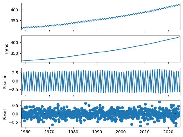
../../../_images/examples_notebooks_generated_stl_seasonal_diagnostic_plot_3_0.png

Looks great! But notice that we did not set the seasonal parameter, even though we know that we’re supposed to. How can we ever know what value we should set it to?

Let’s first explore what the seasonal parameter does and then use a graphical technique to help us decide what value we should set it to.

What is the `seasonal` parameter?¶

The STL method is described in a 1990 paper by Cleveland et al. They propose an iterated inner loop that smooths the seasonal and trend parameters and an outer loop that can be used to provide robustness. Let’s read the original source:

Suppose the number of observations in each period, or cycle, of the seasonal component is \(n_{(p)}\). For example, if the series is monthly with a yearly periodicity, then \(n_{(p)}=12\). We need to be able to refer to the subseries of values at each position of the seasonal cycle. For example, for a monthly series with \(n_{(p)}=12\), the first subseries is the January values, the second is the February values, and so forth. We will refer to each of these \(n_{(p)}\) subseries as a cycle-subseries.

[…]

Each pass of the inner loop consists of a seasonal smoothing that updates the seasonal component, followed by a trend smoothing that updates the trend component.

[…]

Cycle-subseries Smoothing. Each cycle-subseries of the detrended series is smoothed by loess with \(q=n_{(s)}\) and \(d=1\).

So let’s proceed with our data and do as the authors say. We’ll take the detrended series and extract each seasonal component. Then let’s graph them to look at them.

[4]:

detrended = co2 - res.trend
seasonal_subcycles = detrended.groupby(lambda ix: ix.month)

Fantastic, we have our seasonal subcycles. But now let’s smooth them using a loess regression with the seasonal parameter we defined earlier.

In the statsmodels version of lowess, the bandwidth parameter is defined as a fraction of the total number of observations, not as a fixed number.

[5]:

smooth_subcycles = []

for month, seasonal_subcycle in seasonal_subcycles:
    ss_ = sl.lowess(
        seasonal_subcycle,
        seasonal_subcycle.index,
        frac=7 / seasonal_subcycle.size,
        return_sorted=False,
    )
    ss = pd.Series(ss_, seasonal_subcycle.index)
    smooth_subcycles.append((month, ss))

Finally, let’s compare them side by side so we can get a good idea of what is happening to each of these subcycles.

[6]:

fig, (ax1, ax2) = mpl.pyplot.subplots(nrows=1, ncols=2, figsize=[12, 4], sharey=True)
for (mth, seasonl), (mth_, smooths) in zip(seasonal_subcycles, smooth_subcycles):
    ax1.plot(seasonl.index, seasonl, label=calendar.month_name[mth])
    ax2.plot(smooths.index, smooths, label=calendar.month_name[mth_])
_ = ax1.legend(loc="upper center", bbox_to_anchor=(1, -0.1), ncols=6)

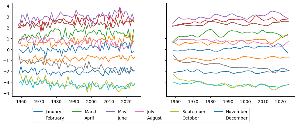
../../../_images/examples_notebooks_generated_stl_seasonal_diagnostic_plot_9_0.png

Of course, each of the subcycles is now much less jumpy than it used to be. The idea, you can probably see already, is that if we look at the seasonal component of our decomposition, we should see each seasonal subcycle develop reasonably smoothly.

What should the `seasonal` parameter be?¶

So we see that the higher the seasonal parameter, the smoother the seasonal subcycles. But on the other hand, if the seasonal parameter is too high, we may fail to capture some evolution in the seasonal cycle. For example, if we look at our data above, we may want to capture the fact that the August series is increasing in magnitude, or what could be maybe an inverted u shape in May. To do that, let’s take a look at a plot suggested by Cleveland et al. called the Seasonal-Diagnostic Plot.

[7]:

from statsmodels.graphics.tsaplots import seasonal_diagnostic_plot

[8]:

# The series starts in March.
months = [
    "March",
    "April",
    "May",
    "June",
    "July",
    "August",
    "September",
    "October",
    "November",
    "December",
    "January",
    "February",
]
fig = seasonal_diagnostic_plot(res, period=12, nrows=3, labels=months)
for ax in fig.get_axes():
    xax = ax.xaxis
    xax.set_major_locator(mpl.dates.YearLocator(20))
    xax.set_minor_locator(mpl.ticker.AutoMinorLocator())
_ = fig.suptitle("Decomposition with `seasonal=7`", y=1.05)

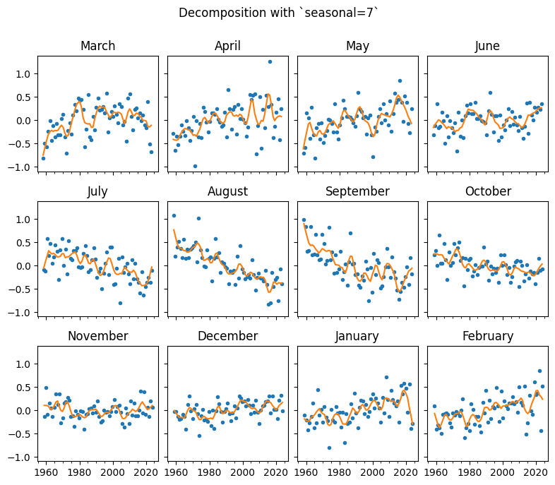
../../../_images/examples_notebooks_generated_stl_seasonal_diagnostic_plot_12_0.png

This plot is similar to the one we did ourselves above to visualise the smoothed cycles, but you can see that the data is now centered at zero, and that each separate seasonal subcycle is plotted against the observations of the data.

More importantly, we can see that each seasonal subcycle is quite noisy, and we may suspect that this noisiness does not reflect the actual evolution of the seasonal component of the series. Let’s see how this compares to the Seasonal-Diagnostic Plot of a series decomposed with a higher seasonal parameter.

[9]:

stl_41 = STL(co2, seasonal=41)
res_41 = stl_41.fit()
fig = seasonal_diagnostic_plot(res_41, period=12, nrows=3, labels=months)
for ax in fig.get_axes():
    xax = ax.xaxis
    xax.set_major_locator(mpl.dates.YearLocator(20))
    xax.set_minor_locator(mpl.ticker.AutoMinorLocator())
_ = fig.suptitle("Decomposition with `seasonal=41`", y=1.05)

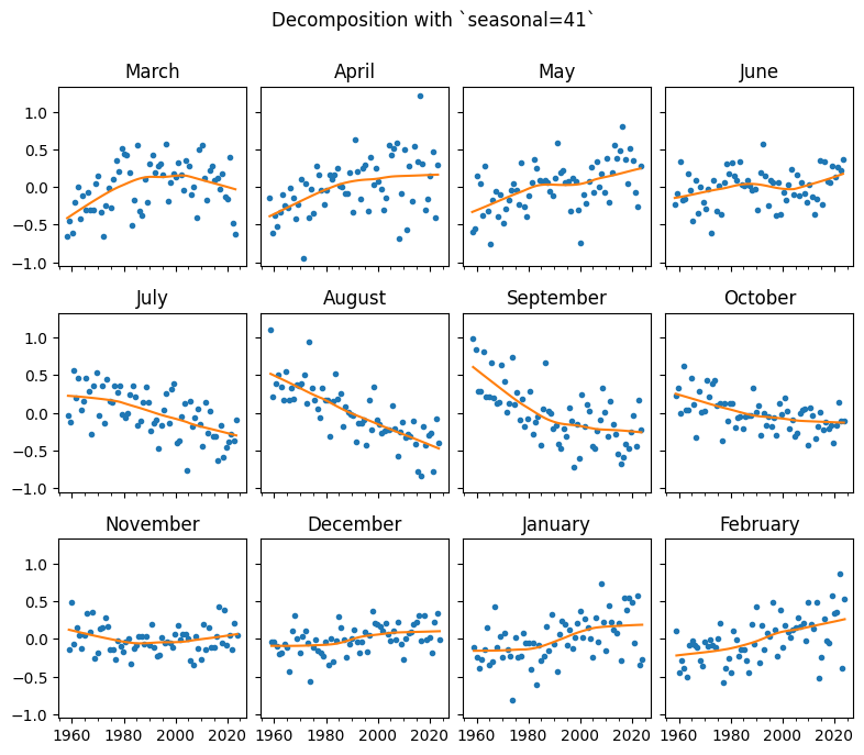
../../../_images/examples_notebooks_generated_stl_seasonal_diagnostic_plot_14_0.png

The observations remain the same, of course, but we can see now that the cycle subseries are much smoother. At the limit, with a high enough seasonal parameter, each of these will be a straight regression line. It is your judgement to decide based on this and your knowledge of the specific data series how you would like the seasonal component to evolve. The value of this parameter here looks right to me because it is evolving smoothly without year-to-year noise, but I still don’t necessarily expect it to be a straight line.

Let’s finish this by comparing each of the components of the decomposition for this data with seasonal=41 and seasonal=7.

[10]:

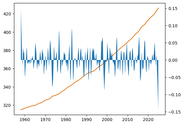
fig, ax1 = mpl.pyplot.subplots()
ax1.plot(res.trend.index, res.trend)
ax1.plot(res.trend.index, res_41.trend)
ax2 = ax1.twinx()
_ = ax2.fill_between(res.trend.index, res.trend - res_41.trend)

../../../_images/examples_notebooks_generated_stl_seasonal_diagnostic_plot_16_0.png

[11]:

fig, (ax1, ax2) = mpl.pyplot.subplots(nrows=2, ncols=1, sharex=True)
ax1.plot(res.seasonal.index, res.seasonal)
ax1.set_title("seasonal=7")
ax2.plot(res_41.seasonal.index, res_41.seasonal)
_ = ax2.set_title("seasonal=41")

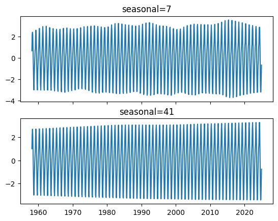
../../../_images/examples_notebooks_generated_stl_seasonal_diagnostic_plot_17_0.png

What a difference that makes! The trend line is basically indistinguishable, but the seasonal parameter has a much smoother evolution.

You now understand how to use the seasonal parameter to determine how the seasonal component of your decomposed time series will evolve and in the Seasonal-Diagnostic Plot you have a tool to help you do it.

Setting the seasonal value in STL¶

What is the seasonal parameter?¶

What should the seasonal parameter be?¶

Setting the `seasonal` value in STL¶

What is the `seasonal` parameter?¶

What should the `seasonal` parameter be?¶