Trends and cycles in unemployment
Here we consider three methods for separating a trend and cycle in economic data. Supposing we have a time series \(y_t\), the basic idea is to decompose it into these two components:
where \(\mu_t\) represents the trend or level and \(\eta_t\) represents the cyclical component. In this case, we consider a stochastic trend, so that \(\mu_t\) is a random variable and not a deterministic function of time. Two of methods fall under the heading of “unobserved components” models, and the third is the popular Hodrick-Prescott (HP) filter. Consistent with e.g. Harvey and Jaeger (1993), we find that these models all produce similar decompositions.
This notebook demonstrates applying these models to separate trend from cycle in the U.S. unemployment rate.
[1]:
%matplotlib inline
[2]:
import numpy as np
import pandas as pd
import statsmodels.api as sm
import matplotlib.pyplot as plt
[3]:
from pandas_datareader.data import DataReader
endog = DataReader('UNRATE', 'fred', start='1954-01-01')
endog.index.freq = endog.index.inferred_freq
Hodrick-Prescott (HP) filter
The first method is the Hodrick-Prescott filter, which can be applied to a data series in a very straightforward method. Here we specify the parameter \(\lambda=129600\) because the unemployment rate is observed monthly.
[4]:
hp_cycle, hp_trend = sm.tsa.filters.hpfilter(endog, lamb=129600)
Unobserved components and ARIMA model (UC-ARIMA)
The next method is an unobserved components model, where the trend is modeled as a random walk and the cycle is modeled with an ARIMA model - in particular, here we use an AR(4) model. The process for the time series can be written as:
where \(\phi(L)\) is the AR(4) lag polynomial and \(\epsilon_t\) and \(\nu_t\) are white noise.
[5]:
mod_ucarima = sm.tsa.UnobservedComponents(endog, 'rwalk', autoregressive=4)
# Here the powell method is used, since it achieves a
# higher loglikelihood than the default L-BFGS method
res_ucarima = mod_ucarima.fit(method='powell', disp=False)
print(res_ucarima.summary())
                        Unobserved Components Results
==============================================================================
Dep. Variable:                 UNRATE   No. Observations:                  861
Model:                    random walk   Log Likelihood                -466.844
                              + AR(4)   AIC                            945.687
Date:                Fri, 05 Dec 2025   BIC                            974.229
Time:                        18:07:45   HQIC                           956.614
Sample:                    01-01-1954
                         - 09-01-2025
Covariance Type:                  opg
================================================================================
                   coef    std err          z      P>|z|      [0.025      0.975]
--------------------------------------------------------------------------------
sigma2.level     0.0739      0.135      0.546      0.585      -0.191       0.339
sigma2.ar        0.0957      0.138      0.694      0.488      -0.175       0.366
ar.L1            1.0530      0.080     13.144      0.000       0.896       1.210
ar.L2           -0.1822      0.274     -0.664      0.507      -0.720       0.355
ar.L3            0.1217      0.201      0.604      0.546      -0.273       0.517
ar.L4           -0.0401      0.095     -0.424      0.672      -0.226       0.146
===================================================================================
Ljung-Box (L1) (Q):                   0.00   Jarque-Bera (JB):           7022861.71
Prob(Q):                              0.97   Prob(JB):                         0.00
Heteroskedasticity (H):               9.07   Skew:                            17.60
Prob(H) (two-sided):                  0.00   Kurtosis:                       444.30
===================================================================================

Warnings:
[1] Covariance matrix calculated using the outer product of gradients (complex-step).
Unobserved components with stochastic cycle (UC)
The final method is also an unobserved components model, but where the cycle is modeled explicitly.
[6]:
mod_uc = sm.tsa.UnobservedComponents(
    endog, 'rwalk',
    cycle=True, stochastic_cycle=True, damped_cycle=True,
)
# Here the powell method gets close to the optimum
res_uc = mod_uc.fit(method='powell', disp=False)
# but to get to the highest loglikelihood we do a
# second round using the L-BFGS method.
res_uc = mod_uc.fit(res_uc.params, disp=False)
print(res_uc.summary())
                            Unobserved Components Results
=====================================================================================
Dep. Variable:                        UNRATE   No. Observations:                  861
Model:                           random walk   Log Likelihood                -470.282
                   + damped stochastic cycle   AIC                            948.564
Date:                       Fri, 05 Dec 2025   BIC                            967.582
Time:                               18:07:46   HQIC                           955.846
Sample:                           01-01-1954
                                - 09-01-2025
Covariance Type:                         opg
===================================================================================
                      coef    std err          z      P>|z|      [0.025      0.975]
-----------------------------------------------------------------------------------
sigma2.level        0.1752      0.004     47.092      0.000       0.168       0.183
sigma2.cycle     2.185e-11      0.002   9.98e-09      1.000      -0.004       0.004
frequency.cycle     0.3491    532.090      0.001      0.999   -1042.528    1043.226
damping.cycle       0.1108     33.767      0.003      0.997     -66.071      66.292
===================================================================================
Ljung-Box (L1) (Q):                   1.18   Jarque-Bera (JB):           7065137.65
Prob(Q):                              0.28   Prob(JB):                         0.00
Heteroskedasticity (H):               9.67   Skew:                            17.58
Prob(H) (two-sided):                  0.00   Kurtosis:                       446.16
===================================================================================

Warnings:
[1] Covariance matrix calculated using the outer product of gradients (complex-step).
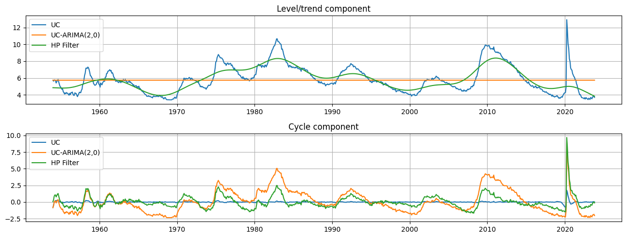
Graphical comparison
The output of each of these models is an estimate of the trend component \(\mu_t\) and an estimate of the cyclical component \(\eta_t\). Qualitatively the estimates of trend and cycle are very similar, although the trend component from the HP filter is somewhat more variable than those from the unobserved components models. This means that relatively mode of the movement in the unemployment rate is attributed to changes in the underlying trend rather than to temporary cyclical movements.
[7]:
fig, axes = plt.subplots(2, figsize=(13,5));
axes[0].set(title='Level/trend component')
axes[0].plot(endog.index, res_uc.level.smoothed, label='UC')
axes[0].plot(endog.index, res_ucarima.level.smoothed, label='UC-ARIMA(2,0)')
axes[0].plot(hp_trend, label='HP Filter')
axes[0].legend(loc='upper left')
axes[0].grid()

axes[1].set(title='Cycle component')
axes[1].plot(endog.index, res_uc.cycle.smoothed, label='UC')
axes[1].plot(endog.index, res_ucarima.autoregressive.smoothed, label='UC-ARIMA(2,0)')
axes[1].plot(hp_cycle, label='HP Filter')
axes[1].legend(loc='upper left')
axes[1].grid()

fig.tight_layout();