Autoregressive Moving Average (ARMA): Sunspots data
[1]:
%matplotlib inline
[2]:
import numpy as np
from scipy import stats
import pandas as pd
import matplotlib.pyplot as plt

import statsmodels.api as sm
from statsmodels.tsa.arima.model import ARIMA
[3]:
from statsmodels.graphics.api import qqplot
Sunspots Data
[4]:
print(sm.datasets.sunspots.NOTE)
::
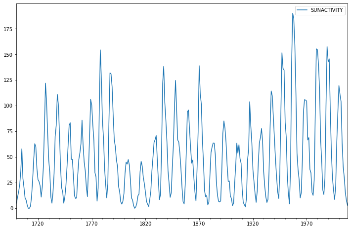
Number of Observations - 309 (Annual 1700 - 2008)
Number of Variables - 1
Variable name definitions::
SUNACTIVITY - Number of sunspots for each year
The data file contains a 'YEAR' variable that is not returned by load.
[5]:
dta = sm.datasets.sunspots.load_pandas().data
[6]:
dta.index = pd.Index(sm.tsa.datetools.dates_from_range('1700', '2008'))
del dta["YEAR"]
[7]:
dta.plot(figsize=(12,8));
[7]:
<AxesSubplot:>
[8]:
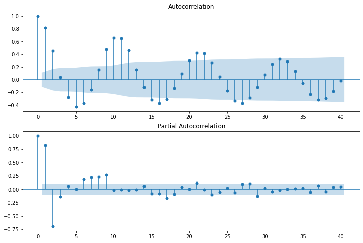
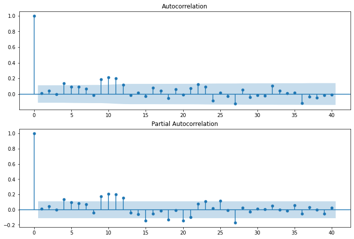
fig = plt.figure(figsize=(12,8))
ax1 = fig.add_subplot(211)
fig = sm.graphics.tsa.plot_acf(dta.values.squeeze(), lags=40, ax=ax1)
ax2 = fig.add_subplot(212)
fig = sm.graphics.tsa.plot_pacf(dta, lags=40, ax=ax2)
[9]:
arma_mod20 = ARIMA(dta, order=(2, 0, 0)).fit()
print(arma_mod20.params)
/home/travis/build/statsmodels/statsmodels/statsmodels/tsa/base/tsa_model.py:527: ValueWarning: No frequency information was provided, so inferred frequency A-DEC will be used.
  % freq, ValueWarning)
/home/travis/build/statsmodels/statsmodels/statsmodels/tsa/base/tsa_model.py:527: ValueWarning: No frequency information was provided, so inferred frequency A-DEC will be used.
  % freq, ValueWarning)
/home/travis/build/statsmodels/statsmodels/statsmodels/tsa/base/tsa_model.py:527: ValueWarning: No frequency information was provided, so inferred frequency A-DEC will be used.
  % freq, ValueWarning)
const      49.746198
ar.L1       1.390633
ar.L2      -0.688573
sigma2    274.727182
dtype: float64
[10]:
arma_mod30 = ARIMA(dta, order=(3, 0, 0)).fit()
/home/travis/build/statsmodels/statsmodels/statsmodels/tsa/base/tsa_model.py:527: ValueWarning: No frequency information was provided, so inferred frequency A-DEC will be used.
  % freq, ValueWarning)
/home/travis/build/statsmodels/statsmodels/statsmodels/tsa/base/tsa_model.py:527: ValueWarning: No frequency information was provided, so inferred frequency A-DEC will be used.
  % freq, ValueWarning)
/home/travis/build/statsmodels/statsmodels/statsmodels/tsa/base/tsa_model.py:527: ValueWarning: No frequency information was provided, so inferred frequency A-DEC will be used.
  % freq, ValueWarning)
[11]:
print(arma_mod20.aic, arma_mod20.bic, arma_mod20.hqic)
2622.637093301343 2637.570458408934 2628.607481146589
[12]:
print(arma_mod30.params)
const      49.751911
ar.L1       1.300818
ar.L2      -0.508102
ar.L3      -0.129644
sigma2    270.101140
dtype: float64
[13]:
print(arma_mod30.aic, arma_mod30.bic, arma_mod30.hqic)
2619.4036292456494 2638.0703356301383 2626.866614052207
Does our model obey the theory?
[14]:
sm.stats.durbin_watson(arma_mod30.resid.values)
[14]:
1.9564953613122156
[15]:
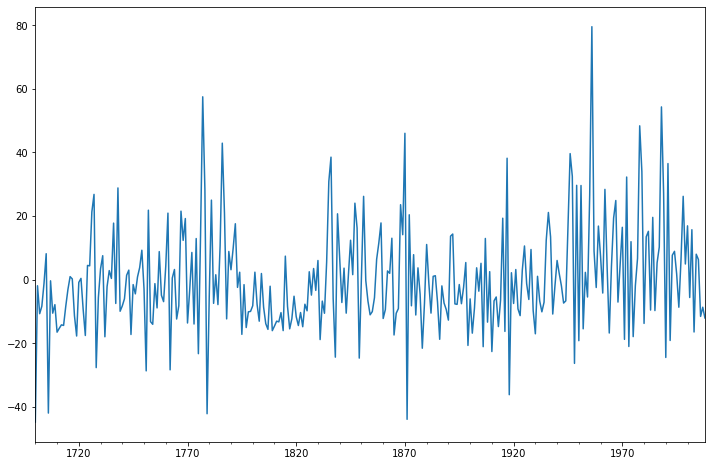
fig = plt.figure(figsize=(12,8))
ax = fig.add_subplot(111)
ax = arma_mod30.resid.plot(ax=ax);
[16]:
resid = arma_mod30.resid
[17]:
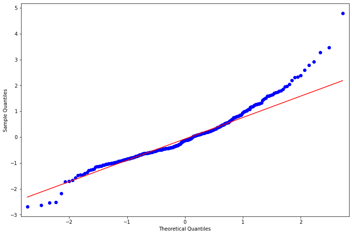
stats.normaltest(resid)
[17]:
NormaltestResult(statistic=49.843932217643335, pvalue=1.5015079664870237e-11)
[18]:
fig = plt.figure(figsize=(12,8))
ax = fig.add_subplot(111)
fig = qqplot(resid, line='q', ax=ax, fit=True)
[19]:
fig = plt.figure(figsize=(12,8))
ax1 = fig.add_subplot(211)
fig = sm.graphics.tsa.plot_acf(resid.values.squeeze(), lags=40, ax=ax1)
ax2 = fig.add_subplot(212)
fig = sm.graphics.tsa.plot_pacf(resid, lags=40, ax=ax2)
[20]:
r,q,p = sm.tsa.acf(resid.values.squeeze(), fft=True, qstat=True)
data = np.c_[range(1,41), r[1:], q, p]
table = pd.DataFrame(data, columns=['lag', "AC", "Q", "Prob(>Q)"])
print(table.set_index('lag'))
            AC          Q      Prob(>Q)
lag
1.0   0.009170   0.026239  8.713184e-01
2.0   0.041793   0.572982  7.508939e-01
3.0  -0.001338   0.573544  9.024612e-01
4.0   0.136086   6.408642  1.706385e-01
5.0   0.092465   9.111351  1.047043e-01
6.0   0.091947  11.792661  6.675737e-02
7.0   0.068747  13.296552  6.520425e-02
8.0  -0.015022  13.368601  9.978086e-02
9.0   0.187590  24.641072  3.394963e-03
10.0  0.213715  39.320758  2.230588e-05
11.0  0.201079  52.359565  2.346490e-07
12.0  0.117180  56.802479  8.580351e-08
13.0 -0.014057  56.866630  1.895209e-07
14.0  0.015398  56.943864  4.000370e-07
15.0 -0.024969  57.147642  7.746546e-07
16.0  0.080916  59.295052  6.876728e-07
17.0  0.041138  59.852008  1.111674e-06
18.0 -0.052022  60.745723  1.549418e-06
19.0  0.062496  62.040010  1.832778e-06
20.0 -0.010303  62.075305  3.383285e-06
21.0  0.074453  63.924941  3.195540e-06
22.0  0.124954  69.152954  8.984238e-07
23.0  0.093162  72.069214  5.803579e-07
24.0 -0.082152  74.344911  4.716006e-07
25.0  0.015696  74.428271  8.294197e-07
26.0 -0.025037  74.641127  1.368121e-06
27.0 -0.125862  80.039434  3.724792e-07
28.0  0.053227  81.008321  4.718979e-07
29.0 -0.038693  81.522151  6.920524e-07
30.0 -0.016903  81.620562  1.152301e-06
31.0 -0.019297  81.749282  1.869783e-06
32.0  0.104990  85.573436  8.932762e-07
33.0  0.040086  86.132924  1.248176e-06
34.0  0.008829  86.160166  2.048904e-06
35.0  0.014589  86.234809  3.265491e-06
36.0 -0.119329  91.247280  1.085015e-06
37.0 -0.036664  91.722221  1.522712e-06
38.0 -0.046193  92.478877  1.939724e-06
39.0 -0.017768  92.591238  2.992188e-06
40.0 -0.006220  92.605057  4.699318e-06
/home/travis/build/statsmodels/statsmodels/statsmodels/tsa/stattools.py:662: FutureWarning: The default number of lags is changing from 40 tomin(int(10 * np.log10(nobs)), nobs - 1) after 0.12is released. Set the number of lags to an integer to  silence this warning.
  FutureWarning,
This indicates a lack of fit.
In-sample dynamic prediction. How good does our model do?
[21]:
predict_sunspots = arma_mod30.predict('1990', '2012', dynamic=True)
print(predict_sunspots)
1990-12-31    167.048337
1991-12-31    140.995022
1992-12-31     94.862115
1993-12-31     46.864439
1994-12-31     11.246106
1995-12-31     -4.718265
1996-12-31     -1.164628
1997-12-31     16.187246
1998-12-31     39.022948
1999-12-31     59.450799
2000-12-31     72.171269
2001-12-31     75.378329
2002-12-31     70.438480
2003-12-31     60.733987
2004-12-31     50.204383
2005-12-31     42.078584
2006-12-31     38.116648
2007-12-31     38.456730
2008-12-31     41.965644
2009-12-31     46.870948
2010-12-31     51.424877
2011-12-31     54.401403
2012-12-31     55.323515
Freq: A-DEC, Name: predicted_mean, dtype: float64
[22]:
def mean_forecast_err(y, yhat):
    return y.sub(yhat).mean()
[23]:
mean_forecast_err(dta.SUNACTIVITY, predict_sunspots)
[23]:
5.634832993585241
Exercise: Can you obtain a better fit for the Sunspots model? (Hint: sm.tsa.AR has a method select_order)
Simulated ARMA(4,1): Model Identification is Difficult
[24]:
from statsmodels.tsa.arima_process import ArmaProcess
[25]:
np.random.seed(1234)
# include zero-th lag
arparams = np.array([1, .75, -.65, -.55, .9])
maparams = np.array([1, .65])
Let’s make sure this model is estimable.
[26]:
arma_t = ArmaProcess(arparams, maparams)
[27]:
arma_t.isinvertible
[27]:
True
[28]:
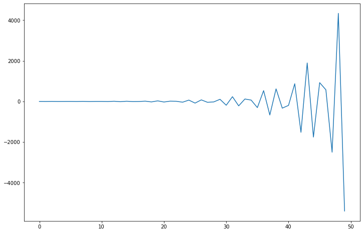
arma_t.isstationary
[28]:
False
What does this mean?
[29]:
fig = plt.figure(figsize=(12,8))
ax = fig.add_subplot(111)
ax.plot(arma_t.generate_sample(nsample=50));
[29]:
[<matplotlib.lines.Line2D at 0x7f85b00f7bd0>]
[30]:
arparams = np.array([1, .35, -.15, .55, .1])
maparams = np.array([1, .65])
arma_t = ArmaProcess(arparams, maparams)
arma_t.isstationary
[30]:
True
[31]:
arma_rvs = arma_t.generate_sample(nsample=500, burnin=250, scale=2.5)
[32]:
fig = plt.figure(figsize=(12,8))
ax1 = fig.add_subplot(211)
fig = sm.graphics.tsa.plot_acf(arma_rvs, lags=40, ax=ax1)
ax2 = fig.add_subplot(212)
fig = sm.graphics.tsa.plot_pacf(arma_rvs, lags=40, ax=ax2)
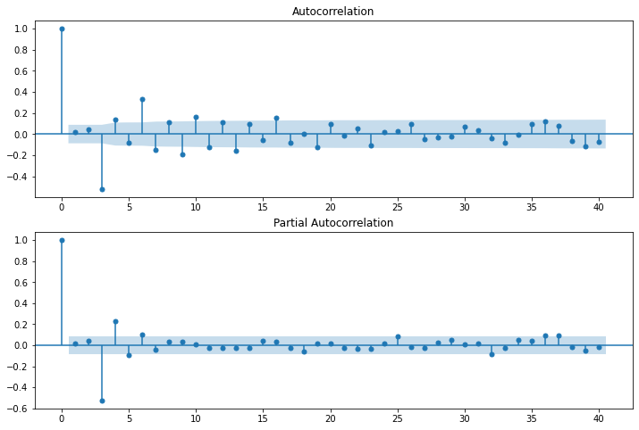
For mixed ARMA processes the Autocorrelation function is a mixture of exponentials and damped sine waves after (q-p) lags.
The partial autocorrelation function is a mixture of exponentials and dampened sine waves after (p-q) lags.
[33]:
arma11 = ARIMA(arma_rvs, order=(1, 0, 1)).fit()
resid = arma11.resid
r,q,p = sm.tsa.acf(resid, fft=True, qstat=True)
data = np.c_[range(1,41), r[1:], q, p]
table = pd.DataFrame(data, columns=['lag', "AC", "Q", "Prob(>Q)"])
print(table.set_index('lag'))
/home/travis/build/statsmodels/statsmodels/statsmodels/tsa/statespace/sarimax.py:966: UserWarning: Non-stationary starting autoregressive parameters found. Using zeros as starting parameters.
  warn('Non-stationary starting autoregressive parameters'
/home/travis/build/statsmodels/statsmodels/statsmodels/tsa/statespace/sarimax.py:978: UserWarning: Non-invertible starting MA parameters found. Using zeros as starting parameters.
  warn('Non-invertible starting MA parameters found.'
            AC           Q      Prob(>Q)
lag
1.0  -0.001244    0.000778  9.777436e-01
2.0   0.052350    1.382049  5.010626e-01
3.0  -0.522181  139.090106  5.938063e-30
4.0   0.146506  149.951983  2.084573e-31
5.0  -0.091171  154.166872  1.731083e-31
6.0   0.337059  211.891306  5.568290e-43
7.0  -0.160920  225.075262  5.519054e-45
8.0   0.116132  231.955610  1.142179e-45
9.0  -0.195352  251.464207  4.895752e-49
10.0  0.166410  265.649428  2.760836e-51
11.0 -0.126465  273.858717  2.767679e-52
12.0  0.115015  280.662675  5.334652e-53
13.0 -0.159302  293.742050  4.899046e-55
14.0  0.095846  298.486519  2.444596e-55
15.0 -0.062853  300.531001  4.335557e-55
16.0  0.159244  313.681886  3.718133e-57
17.0 -0.089423  317.837389  2.317190e-57
18.0  0.002504  317.840655  1.018533e-56
19.0 -0.124735  325.959706  9.297882e-58
20.0  0.093960  330.576238  4.414194e-58
21.0 -0.016212  330.713971  1.708363e-57
22.0  0.054804  332.291098  3.279536e-57
23.0 -0.110592  338.726892  6.325402e-58
24.0  0.022742  338.999620  2.166837e-57
25.0  0.029459  339.458216  6.665490e-57
26.0  0.095294  344.266902  2.658405e-57
27.0 -0.053408  345.780570  4.853849e-57
28.0 -0.029575  346.245693  1.418122e-56
29.0 -0.022668  346.519521  4.448333e-56
30.0  0.066872  348.907686  5.186512e-56
31.0  0.039120  349.726701  1.228743e-55
32.0 -0.041051  350.630508  2.760218e-55
33.0 -0.084511  354.469188  1.602581e-55
34.0 -0.008108  354.504597  5.223692e-55
35.0  0.090451  358.920813  2.295026e-55
36.0  0.118710  366.543846  2.342022e-56
37.0  0.074002  369.512605  1.968357e-56
38.0 -0.067954  372.021404  2.022311e-56
39.0 -0.116515  379.412938  2.277599e-57
40.0 -0.071747  382.221721  2.023659e-57
/home/travis/build/statsmodels/statsmodels/statsmodels/tsa/stattools.py:662: FutureWarning: The default number of lags is changing from 40 tomin(int(10 * np.log10(nobs)), nobs - 1) after 0.12is released. Set the number of lags to an integer to  silence this warning.
  FutureWarning,
[34]:
arma41 = ARIMA(arma_rvs, order=(4, 0, 1)).fit()
resid = arma41.resid
r,q,p = sm.tsa.acf(resid, fft=True, qstat=True)
data = np.c_[range(1,41), r[1:], q, p]
table = pd.DataFrame(data, columns=['lag', "AC", "Q", "Prob(>Q)"])
print(table.set_index('lag'))
            AC          Q  Prob(>Q)
lag
1.0  -0.007899   0.031383  0.859389
2.0   0.004128   0.039972  0.980212
3.0   0.018095   0.205341  0.976722
4.0  -0.006766   0.228509  0.993949
5.0   0.018123   0.395044  0.995465
6.0   0.050690   1.700565  0.945078
7.0   0.010253   1.754087  0.972191
8.0  -0.011208   1.818176  0.986088
9.0   0.020292   2.028663  0.991006
10.0  0.001028   2.029204  0.996111
11.0 -0.014033   2.130285  0.997983
12.0 -0.023858   2.423052  0.998426
13.0 -0.002108   2.425342  0.999339
14.0 -0.018784   2.607562  0.999589
15.0  0.011317   2.673844  0.999805
16.0  0.042158   3.595554  0.999443
17.0  0.007943   3.628344  0.999734
18.0 -0.074312   6.504019  0.993685
19.0 -0.023378   6.789205  0.995255
20.0  0.002398   6.792213  0.997313
21.0  0.000488   6.792338  0.998515
22.0  0.017953   6.961578  0.999024
23.0 -0.038576   7.744617  0.998744
24.0 -0.029817   8.213410  0.998859
25.0  0.077850  11.415980  0.990674
26.0  0.040407  12.280577  0.989478
27.0 -0.018613  12.464413  0.992261
28.0 -0.014765  12.580339  0.994586
29.0  0.017650  12.746347  0.996111
30.0 -0.005486  12.762422  0.997504
31.0  0.058257  14.578761  0.994613
32.0 -0.040841  15.473357  0.993886
33.0 -0.019495  15.677617  0.995392
34.0  0.037267  16.425688  0.995214
35.0  0.086212  20.437647  0.976294
36.0  0.041271  21.359026  0.974772
37.0  0.078704  24.717091  0.938945
38.0 -0.029731  25.197309  0.944891
39.0 -0.078398  28.543746  0.891169
40.0 -0.014466  28.657935  0.909260
/home/travis/build/statsmodels/statsmodels/statsmodels/tsa/stattools.py:662: FutureWarning: The default number of lags is changing from 40 tomin(int(10 * np.log10(nobs)), nobs - 1) after 0.12is released. Set the number of lags to an integer to  silence this warning.
  FutureWarning,
Exercise: How good of in-sample prediction can you do for another series, say, CPI
[35]:
macrodta = sm.datasets.macrodata.load_pandas().data
macrodta.index = pd.Index(sm.tsa.datetools.dates_from_range('1959Q1', '2009Q3'))
cpi = macrodta["cpi"]
Hint:
[36]:
fig = plt.figure(figsize=(12,8))
ax = fig.add_subplot(111)
ax = cpi.plot(ax=ax);
ax.legend();
[36]:
<matplotlib.legend.Legend at 0x7f85abee2410>
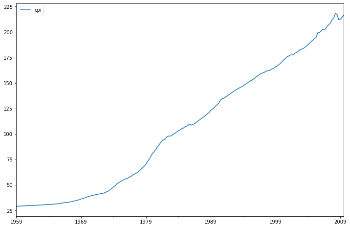
P-value of the unit-root test, resoundingly rejects the null of a unit-root.
[37]:
print(sm.tsa.adfuller(cpi)[1])
0.9904328188337421