statsmodels.graphics.tsaplots.seasonal_diagnostic_plot#

statsmodels.graphics.tsaplots.seasonal_diagnostic_plot(x, period, subplots=None, labels=None, nrows=1, **kwargs)[source]#

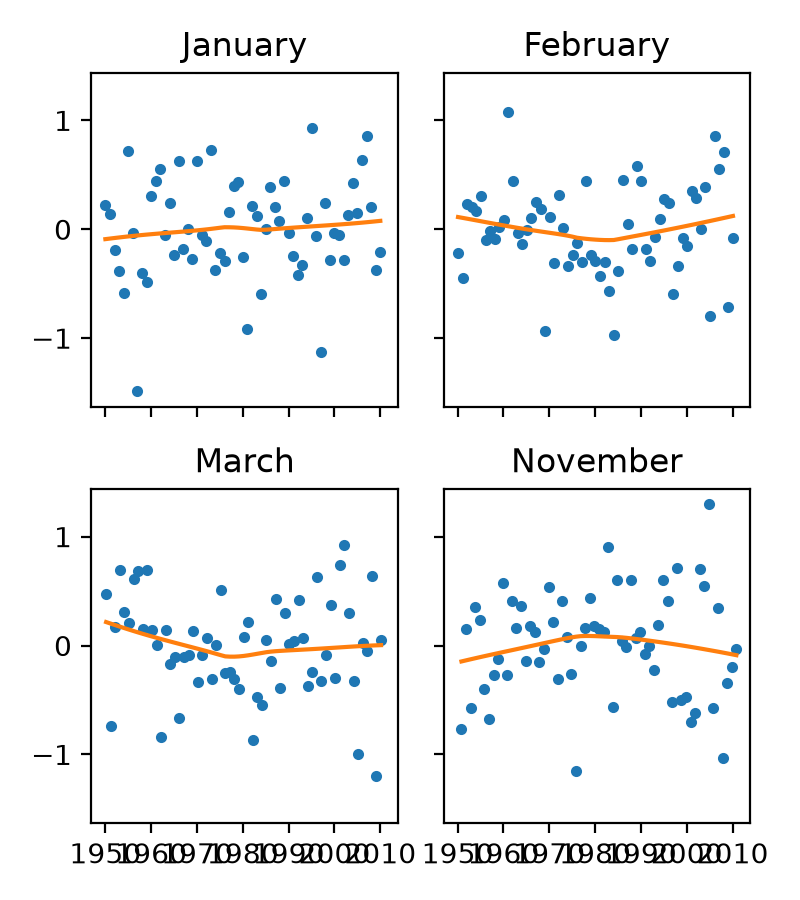
Seasonal-Diagnostic Plot, as described by [1]

Parameters:

xDecomposeResult: The result of your seasonal decomposition.
periodint: The length of the period. Should match the period parameter used to decompose the series.
subplotsint, list of int, or ndarray of int, optional: If period is large, subplots can be used to specify how many should be plotted. If subplots is an int, the periods are selected evenly from range(period). If subplots is a list or ndarray of int, the periods with those indices will be selected for the subplots. By default, subplots=period.
labelssequence of str, optional: Labels for the displayed period subplots.
nrowsint, optional: The number of rows on which to display the plots.
**kwargs: Additional keyword arguments passed to plt.subplots, such as figsize or ncols.

Returns:

figFigure: Returns a matplotlib object of type Figure with the Seasonal-Diagnostic Plot.

References

[1]

Cleveland, Robert B., William S. Cleveland, Jean E. McRae, Irma Terpenning (1990) “STL: A Seasonal-Trend Decomposition Procedure Based on Loess”. Journal of Official Statistics, 6 (1), 3-33.

Examples

>>> from statsmodels.datasets import co2
>>> from statsmodels.tsa.seasonal import STL
>>> from statsmodels.graphics.tsaplots import seasonal_diagnostic_plot

>>> data = (co2.load().data
...         .loc[lambda df: df.index.isocalendar().week<53]
...         .loc['1986-01-01':]
... )

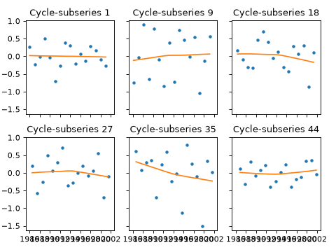
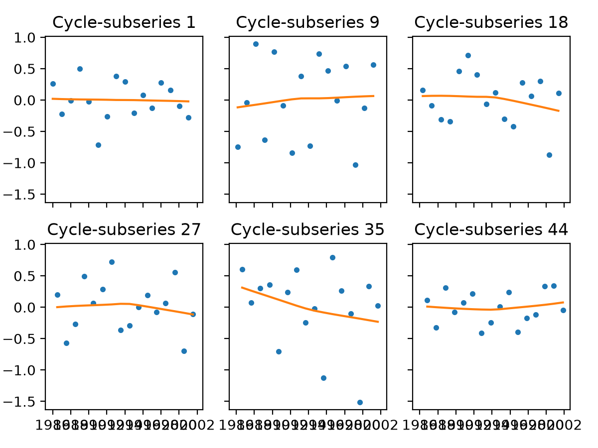
>>> res = STL(data, period=52, seasonal=21).fit()
>>> _ = seasonal_diagnostic_plot(res, period=52, subplots=6, nrows=2)

(Source code, png, hires.png, pdf)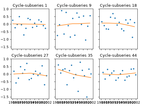

>>> from statsmodels.datasets import elnino
>>> from statsmodels.tsa.seasonal import STL
>>> from statsmodels.graphics.tsaplots import seasonal_diagnostic_plot
>>> import pandas as pd

>>> month_dict = {'JAN':1, 'FEB':2, 'MAR':3, 'APR':4, 'MAY':5, 'JUN':6,
...               'JUL':7, 'AUG':8, 'SEP':9, 'OCT':10, 'NOV':11, 'DEC':12}
>>> data = (elnino.load().data
...    .rename(columns=month_dict)
...    .melt(id_vars=['YEAR'], var_name='month')
...    .assign(day=1,
...            date = lambda df: pd.to_datetime(
...                    df[['YEAR', 'month', 'day']]))
...    .drop(columns=['YEAR', 'month', 'day'])
...    .set_index('date')
...    .sort_index()
...   )

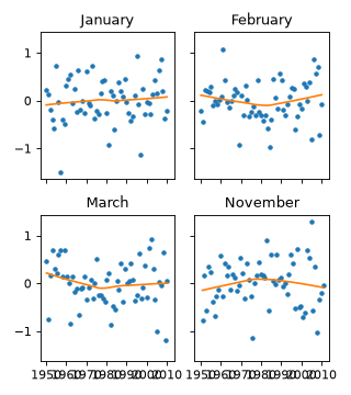
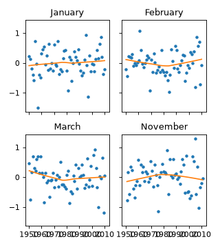
>>> res = STL(data, period=12, seasonal=53).fit()
>>> labels=['January', 'February', 'March', 'November']
>>> _ = seasonal_diagnostic_plot(res, period=12, subplots=[0,1,2,10],
...                              labels=labels, nrows=2)

(Source code, png, hires.png, pdf)