
statsmodels.tsa.filters.hamilton_filter.hamilton_filter#
- statsmodels.tsa.filters.hamilton_filter.hamilton_filter(x, h=8, p=4)[source]#
Hamilton (2018) regression-based trend-cycle decomposition.
- Parameters:
- xarray_like
The time series to decompose, 1-d or 2-d with at least
2 p + hobservations- h
int,optional Forecast horizon used in the projection. Hamilton recommends:
8 for quarterly data (two years ahead, default)
24 for monthly data (two years ahead)
2 for annual data
- p
int,optional Number of lagged values of
xto include as regressors. Hamilton recommends 4 for quarterly data (one year of lags), 12 for monthly data (one year of lags), and 1 for annual data (following the same one-year-of-lags rule).
- Returns:
CycleTrendResultA result object with fields:
- cyclendarray, Series, or DataFrame
Estimated cyclical component. The first
p + h - 1values areNaNbecause no regression can be formed for those periods.- trendndarray, Series, or DataFrame
Estimated trend component. The first
p + h - 1values are likewiseNaN.
See also
statsmodels.tsa.filters.hp_filter.hpfilterHodrick-Prescott filter.
statsmodels.tsa.filters.bk_filter.bkfilterBaxter-King bandpass filter.
statsmodels.tsa.filters.cf_filter.cffilterChristiano-Fitzgerald asymmetric filter.
statsmodels.tsa.ar_model.AutoRegAutoregression estimation using OLS.
Notes
Decomposes a time series into trend and cycle components by projecting
h-period-ahead values on thepmost recent lags and a constant:\[y_{t+h} = \alpha_0 + \alpha_1 y_t + \alpha_2 y_{t-1} + \cdots + \alpha_p y_{t-p+1} + v_{t+h}\]The cycle at time
t + his the residual \(\hat{v}_{t+h}\) from this OLS regression. The trend is the corresponding fitted value.Unlike the HP filter, the Hamilton filter uses only lagged information and produces stationary residuals when the underlying series is I(1) or I(2). [Hamilton2018] shows that the HP filter introduces spurious cyclical dynamics; the regression-based filter avoids this by construction.
The regression is estimated once on all available observations (i.e., this is not a rolling regression). With
h = 8andp = 4(the quarterly defaults), the first11observations of the output areNaN.xmust have at least2 * p + hobservations so that the regression has at leastp + 1usable observations (one per parameter, including the constant). At exactly this minimum length, the regression is exactly determined and produces a degenerate, zero-residual fit – the returnedcycleis identically zero andtrendequalsxover the non-NaNrange. Provide more observations than this bare minimum for a meaningful decomposition.References
[Hamilton2018]Hamilton, J. D. (2018). Why You Should Never Use the Hodrick-Prescott Filter. Review of Economics and Statistics, 100(5), 831-843.
Examples
>>> import statsmodels.api as sm
>>> import pandas as pd
>>> dta = sm.datasets.macrodata.load_pandas().data
>>> index = pd.period_range('1959Q1', '2009Q3', freq='Q')
>>> dta.set_index(index, inplace=True)
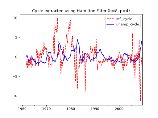
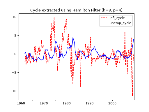
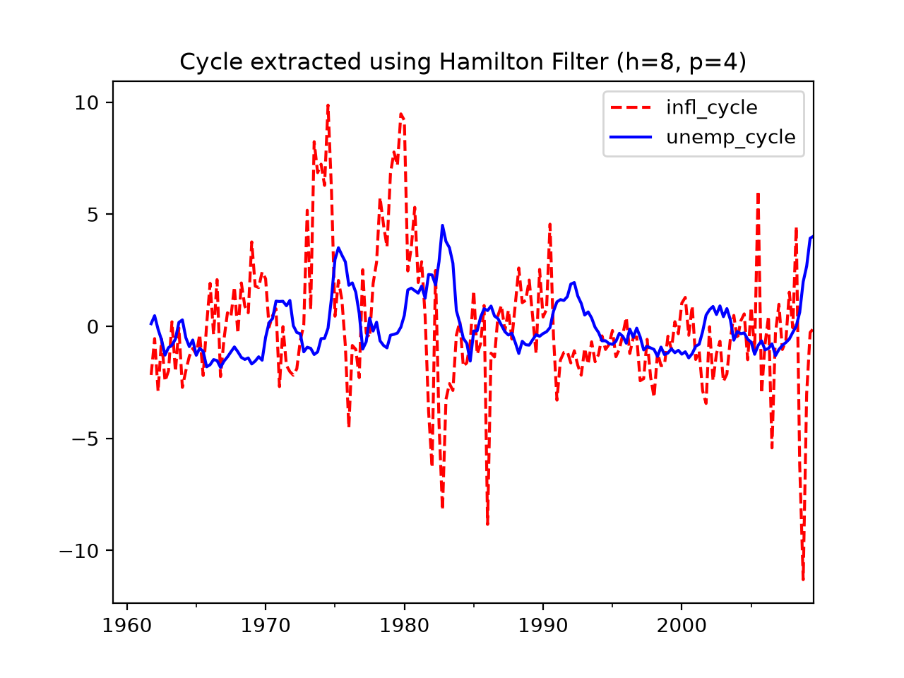
>>> cycle, trend = sm.tsa.filters.hamilton_filter(dta[["infl", "unemp"]], h=8, p=4)
>>> import matplotlib.pyplot as plt
>>> fig, ax = plt.subplots()
>>> cycle.plot(ax=ax, style=['r--', 'b-'])
>>> ax.set_title("Cycle extracted using Hamilton Filter (h=8, p=4)")
>>> plt.show()
(
Source code,png,hires.png,pdf)