Kernel Density Estimation

Kernel density estimation is the process of estimating an unknown probability density function using a kernel function \(K(u)\). While a histogram counts the number of data points in somewhat arbitrary regions, a kernel density estimate is a function defined as the sum of a kernel function on every data point. The kernel function typically exhibits the following properties:

1. Symmetry such that \(K(u) = K(-u)\).

2. Normalization such that \(\int_{-\infty}^{\infty} K(u) \ du = 1\) .

3. Monotonically decreasing such that \(K'(u) < 0\) when \(u > 0\).

4. Expected value equal to zero such that \(\mathrm{E}[K] = 0\).

For more information about kernel density estimation, see for instance Wikipedia - Kernel density estimation.

A univariate kernel density estimator is implemented in sm.nonparametric.KDEUnivariate. In this example we will show the following:

• Basic usage, how to fit the estimator.

• The effect of varying the bandwidth of the kernel using the bw argument.

• The various kernel functions available using the kernel argument.

%matplotlib inline
import matplotlib.pyplot as plt
import numpy as np
from scipy import stats

import statsmodels.api as sm
from statsmodels.distributions.mixture_rvs import mixture_rvs

A univariate example

np.random.seed(12345)  # Seed the random number generator for reproducible results

We create a bimodal distribution: a mixture of two normal distributions with locations at -1 and 1.

# Location, scale and weight for the two distributions
dist1_loc, dist1_scale, weight1 = -1, 0.5, 0.25
dist2_loc, dist2_scale, weight2 = 1, 0.5, 0.75

# Sample from a mixture of distributions
obs_dist = mixture_rvs(
    prob=[weight1, weight2],
    size=250,
    dist=[stats.norm, stats.norm],
    kwargs=(
        dict(loc=dist1_loc, scale=dist1_scale),
        dict(loc=dist2_loc, scale=dist2_scale),
    ),
)

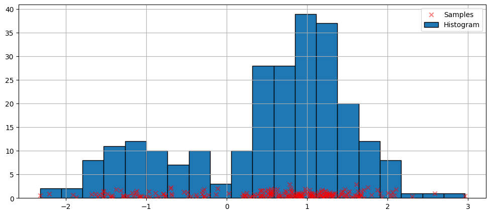
The simplest non-parametric technique for density estimation is the histogram.

fig = plt.figure(figsize=(12, 5))
ax = fig.add_subplot(111)

# Scatter plot of data samples and histogram
ax.scatter(
    obs_dist,
    np.abs(np.random.randn(obs_dist.size)),
    zorder=15,
    color="red",
    marker="x",
    alpha=0.5,
    label="Samples",
)
lines = ax.hist(obs_dist, bins=20, edgecolor="k", label="Histogram")

ax.legend(loc="best")
ax.grid(True, zorder=-5)

Fitting with the default arguments

The histogram above is discontinuous. To compute a continuous probability density function, we can use kernel density estimation.

We initialize a univariate kernel density estimator using KDEUnivariate.

kde = sm.nonparametric.KDEUnivariate(obs_dist)
kde.fit()  # Estimate the densities

<statsmodels.nonparametric.kde.KDEUnivariate at 0x7f9cc6caa3c0>

We present a figure of the fit, as well as the true distribution.

fig = plt.figure(figsize=(12, 5))
ax = fig.add_subplot(111)

# Plot the histogram
ax.hist(
    obs_dist,
    bins=20,
    density=True,
    label="Histogram from samples",
    zorder=5,
    edgecolor="k",
    alpha=0.5,
)

# Plot the KDE as fitted using the default arguments
ax.plot(kde.support, kde.density, lw=3, label="KDE from samples", zorder=10)

# Plot the true distribution
true_values = (
    stats.norm.pdf(loc=dist1_loc, scale=dist1_scale, x=kde.support) * weight1
    + stats.norm.pdf(loc=dist2_loc, scale=dist2_scale, x=kde.support) * weight2
)
ax.plot(kde.support, true_values, lw=3, label="True distribution", zorder=15)

# Plot the samples
ax.scatter(
    obs_dist,
    np.abs(np.random.randn(obs_dist.size)) / 40,
    marker="x",
    color="red",
    zorder=20,
    label="Samples",
    alpha=0.5,
)

ax.legend(loc="best")
ax.grid(True, zorder=-5)

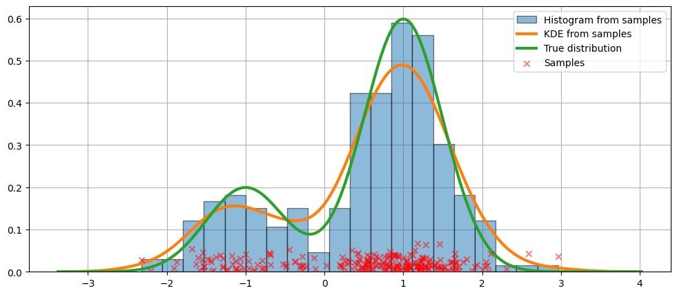
In the code above, default arguments were used. We can also vary the bandwidth of the kernel, as we will now see.

Varying the bandwidth using the bw argument

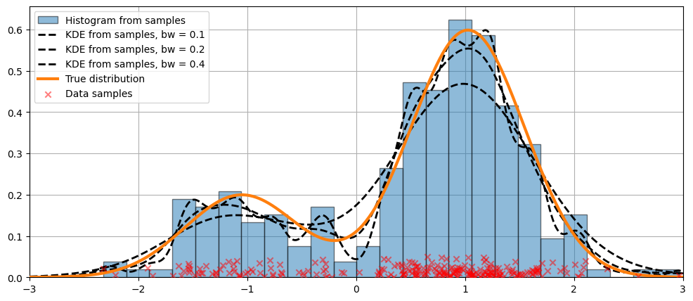
The bandwidth of the kernel can be adjusted using the bw argument. In the following example, a bandwidth of bw=0.2 seems to fit the data well.

fig = plt.figure(figsize=(12, 5))
ax = fig.add_subplot(111)

# Plot the histogram
ax.hist(
    obs_dist,
    bins=25,
    label="Histogram from samples",
    zorder=5,
    edgecolor="k",
    density=True,
    alpha=0.5,
)

# Plot the KDE for various bandwidths
for bandwidth in [0.1, 0.2, 0.4]:
    kde.fit(bw=bandwidth)  # Estimate the densities
    ax.plot(
        kde.support,
        kde.density,
        "--",
        lw=2,
        color="k",
        zorder=10,
        label="KDE from samples, bw = {}".format(round(bandwidth, 2)),
    )

# Plot the true distribution
ax.plot(kde.support, true_values, lw=3, label="True distribution", zorder=15)

# Plot the samples
ax.scatter(
    obs_dist,
    np.abs(np.random.randn(obs_dist.size)) / 50,
    marker="x",
    color="red",
    zorder=20,
    label="Data samples",
    alpha=0.5,
)

ax.legend(loc="best")
ax.set_xlim([-3, 3])
ax.grid(True, zorder=-5)

Comparing kernel functions

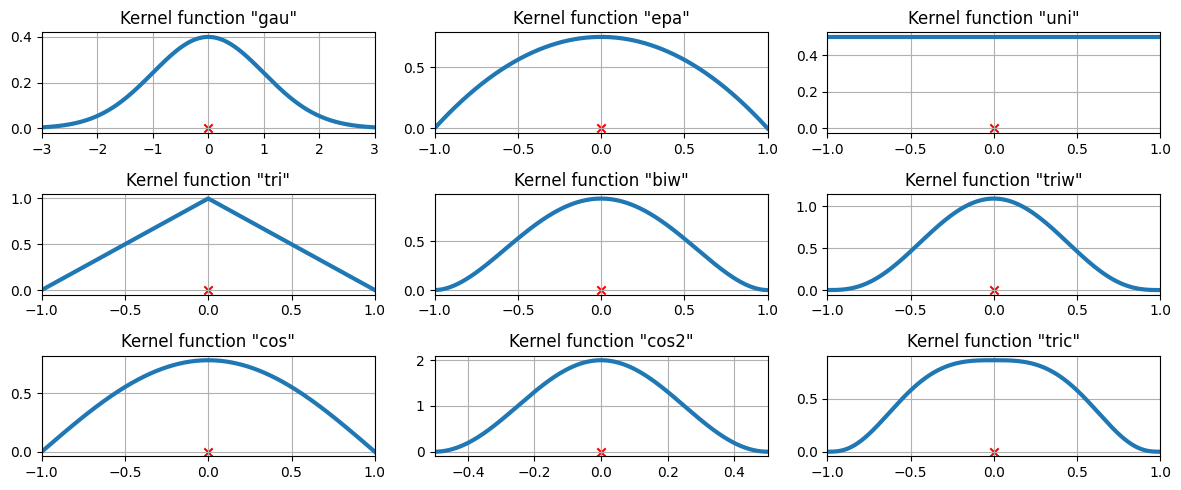
In the example above, a Gaussian kernel was used. Several other kernels are also available.

from statsmodels.nonparametric.kde import kernel_switch

list(kernel_switch.keys())

['gau', 'epa', 'uni', 'tri', 'biw', 'triw', 'cos', 'cos2', 'tric']

The available kernel functions

# Create a figure
fig = plt.figure(figsize=(12, 5))

# Enumerate every option for the kernel
for i, (ker_name, ker_class) in enumerate(kernel_switch.items()):

    # Initialize the kernel object
    kernel = ker_class()

    # Sample from the domain
    domain = kernel.domain or [-3, 3]
    x_vals = np.linspace(*domain, num=2**10)
    y_vals = kernel(x_vals)

    # Create a subplot, set the title
    ax = fig.add_subplot(3, 3, i + 1)
    ax.set_title('Kernel function "{}"'.format(ker_name))
    ax.plot(x_vals, y_vals, lw=3, label="{}".format(ker_name))
    ax.scatter([0], [0], marker="x", color="red")
    plt.grid(True, zorder=-5)
    ax.set_xlim(domain)

plt.tight_layout()

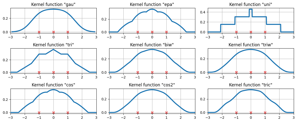
The available kernel functions on three data points

We now examine how the kernel density estimate will fit to three equally spaced data points.

# Create three equidistant points
data = np.linspace(-1, 1, 3)
kde = sm.nonparametric.KDEUnivariate(data)

# Create a figure
fig = plt.figure(figsize=(12, 5))

# Enumerate every option for the kernel
for i, kernel in enumerate(kernel_switch.keys()):

    # Create a subplot, set the title
    ax = fig.add_subplot(3, 3, i + 1)
    ax.set_title('Kernel function "{}"'.format(kernel))

    # Fit the model (estimate densities)
    kde.fit(kernel=kernel, fft=False, gridsize=2**10)

    # Create the plot
    ax.plot(kde.support, kde.density, lw=3, label="KDE from samples", zorder=10)
    ax.scatter(data, np.zeros_like(data), marker="x", color="red")
    plt.grid(True, zorder=-5)
    ax.set_xlim([-3, 3])

plt.tight_layout()

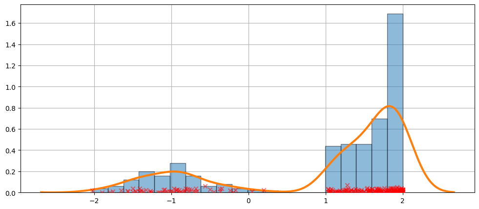
A more difficult case

The fit is not always perfect. See the example below for a harder case.

obs_dist = mixture_rvs(
    [0.25, 0.75],
    size=250,
    dist=[stats.norm, stats.beta],
    kwargs=(dict(loc=-1, scale=0.5), dict(loc=1, scale=1, args=(1, 0.5))),
)

kde = sm.nonparametric.KDEUnivariate(obs_dist)
kde.fit()

<statsmodels.nonparametric.kde.KDEUnivariate at 0x7f9cc15c1450>

fig = plt.figure(figsize=(12, 5))
ax = fig.add_subplot(111)
ax.hist(obs_dist, bins=20, density=True, edgecolor="k", zorder=4, alpha=0.5)
ax.plot(kde.support, kde.density, lw=3, zorder=7)
# Plot the samples
ax.scatter(
    obs_dist,
    np.abs(np.random.randn(obs_dist.size)) / 50,
    marker="x",
    color="red",
    zorder=20,
    label="Data samples",
    alpha=0.5,
)
ax.grid(True, zorder=-5)

The KDE is a distribution

Since the KDE is a distribution, we can access attributes and methods such as:

• entropy

• evaluate

• cdf

• icdf

• sf

• cumhazard

obs_dist = mixture_rvs(
    [0.25, 0.75],
    size=1000,
    dist=[stats.norm, stats.norm],
    kwargs=(dict(loc=-1, scale=0.5), dict(loc=1, scale=0.5)),
)
kde = sm.nonparametric.KDEUnivariate(obs_dist)
kde.fit(gridsize=2**10)

<statsmodels.nonparametric.kde.KDEUnivariate at 0x7f9cc6c92780>

kde.entropy

1.314324140492138

kde.evaluate(-1)

array([0.18085886])

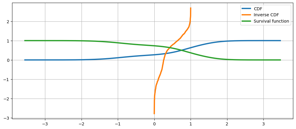
Cumulative distribution, it’s inverse, and the survival function

fig = plt.figure(figsize=(12, 5))
ax = fig.add_subplot(111)

ax.plot(kde.support, kde.cdf, lw=3, label="CDF")
ax.plot(np.linspace(0, 1, num=kde.icdf.size), kde.icdf, lw=3, label="Inverse CDF")
ax.plot(kde.support, kde.sf, lw=3, label="Survival function")
ax.legend(loc="best")
ax.grid(True, zorder=-5)

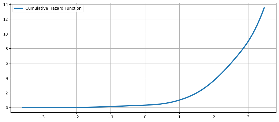
The Cumulative Hazard Function

fig = plt.figure(figsize=(12, 5))
ax = fig.add_subplot(111)
ax.plot(kde.support, kde.cumhazard, lw=3, label="Cumulative Hazard Function")
ax.legend(loc="best")
ax.grid(True, zorder=-5)