

Model Comparison#
This notebook shows how to compare fitted models using the methods that statsmodels provides for the linear regression family (OLS, WLS and GLS).
For any two nested models, statsmodels gives you information criteria (AIC, BIC), likelihood-based tests, and F tests to decide whether a more flexible model is worth the extra parameters. We will fit the three members of the linear regression family to the same dataset and compare them side by side.
[1]:
import matplotlib.pyplot as plt
import numpy as np

import statsmodels.api as sm
The data#
We use the classic Longley dataset, which is bundled with statsmodels. It is a small macroeconomic time series with six predictors and total employment as the response.
[2]:
data = sm.datasets.longley.load()
data.exog = sm.add_constant(data.exog)
print(data.exog.head())
print(data.exog.columns)
   const  GNPDEFL       GNP   UNEMP   ARMED       POP    YEAR
0    1.0     83.0  234289.0  2356.0  1590.0  107608.0  1947.0
1    1.0     88.5  259426.0  2325.0  1456.0  108632.0  1948.0
2    1.0     88.2  258054.0  3682.0  1616.0  109773.0  1949.0
3    1.0     89.5  284599.0  3351.0  1650.0  110929.0  1950.0
4    1.0     96.2  328975.0  2099.0  3099.0  112075.0  1951.0
Index(['const', 'GNPDEFL', 'GNP', 'UNEMP', 'ARMED', 'POP', 'YEAR'], dtype='str')
Baseline: Ordinary Least Squares (OLS)#
The OLS model assumes the errors are independent and identically distributed. It is the natural baseline that the other two estimators generalize.
[3]:
ols_res = sm.OLS(data.endog, data.exog).fit()
print(ols_res.summary())
                            OLS Regression Results
==============================================================================
Dep. Variable:                 TOTEMP   R-squared:                       0.995
Model:                            OLS   Adj. R-squared:                  0.992
Method:                 Least Squares   F-statistic:                     330.3
Date:                Sun, 25 Oct 2026   Prob (F-statistic):           4.98e-10
Time:                        00:22:19   Log-Likelihood:                -109.62
No. Observations:                  16   AIC:                             233.2
Df Residuals:                       9   BIC:                             238.6
Df Model:                           6
Covariance Type:            nonrobust
==============================================================================
                 coef    std err          t      P>|t|      [0.025      0.975]
------------------------------------------------------------------------------
const      -3.482e+06    8.9e+05     -3.911      0.004    -5.5e+06   -1.47e+06
GNPDEFL       15.0619     84.915      0.177      0.863    -177.029     207.153
GNP           -0.0358      0.033     -1.070      0.313      -0.112       0.040
UNEMP         -2.0202      0.488     -4.136      0.003      -3.125      -0.915
ARMED         -1.0332      0.214     -4.822      0.001      -1.518      -0.549
POP           -0.0511      0.226     -0.226      0.826      -0.563       0.460
YEAR        1829.1515    455.478      4.016      0.003     798.788    2859.515
==============================================================================
Omnibus:                        0.749   Durbin-Watson:                   2.559
Prob(Omnibus):                  0.688   Jarque-Bera (JB):                0.684
Skew:                           0.420   Prob(JB):                        0.710
Kurtosis:                       2.434   Cond. No.                     4.86e+09
==============================================================================

Notes:
[1] Standard Errors assume that the covariance matrix of the errors is correctly specified.
[2] The condition number is large, 4.86e+09. This might indicate that there are
strong multicollinearity or other numerical problems.
Weighted Least Squares (WLS)#
If the error variance is not constant but known up to a factor, weighted least squares is more efficient than OLS. The weights are inverse variances, the variance of the error of observation \(i\) is \(\sigma^2 / w_i\). Here we weight each observation by the population (POP), i.e. we assume that the errors of years with a larger population have a smaller variance and trust those observations relatively more. The weights are taken as given, they are not estimated.
[4]:
weights = data.exog["POP"].to_numpy(dtype=float)
wls_res = sm.WLS(data.endog, data.exog, weights=weights).fit()
print(wls_res.summary())
                            WLS Regression Results
==============================================================================
Dep. Variable:                 TOTEMP   R-squared:                       0.995
Model:                            WLS   Adj. R-squared:                  0.992
Method:                 Least Squares   F-statistic:                     331.2
Date:                Sun, 25 Oct 2026   Prob (F-statistic):           4.92e-10
Time:                        00:22:19   Log-Likelihood:                -109.59
No. Observations:                  16   AIC:                             233.2
Df Residuals:                       9   BIC:                             238.6
Df Model:                           6
Covariance Type:            nonrobust
==============================================================================
                 coef    std err          t      P>|t|      [0.025      0.975]
------------------------------------------------------------------------------
const      -3.513e+06   8.92e+05     -3.939      0.003   -5.53e+06    -1.5e+06
GNPDEFL       16.6801     85.244      0.196      0.849    -176.154     209.514
GNP           -0.0368      0.034     -1.094      0.302      -0.113       0.039
UNEMP         -2.0274      0.491     -4.133      0.003      -3.137      -0.918
ARMED         -1.0349      0.215     -4.811      0.001      -1.522      -0.548
POP           -0.0498      0.226     -0.220      0.831      -0.561       0.461
YEAR        1844.6696    456.006      4.045      0.003     813.113    2876.226
==============================================================================
Omnibus:                        0.958   Durbin-Watson:                   2.548
Prob(Omnibus):                  0.619   Jarque-Bera (JB):                0.820
Skew:                           0.478   Prob(JB):                        0.664
Kurtosis:                       2.437   Cond. No.                     4.94e+09
==============================================================================

Notes:
[1] Standard Errors assume that the covariance matrix of the errors is correctly specified.
[2] The condition number is large, 4.94e+09. This might indicate that there are
strong multicollinearity or other numerical problems.
Generalized Least Squares (GLS)#
When the errors are correlated (as is often the case in time series), GLS can take that correlation structure into account. We fit the same model but assume the errors follow an AR(1) process. A consistent estimate of the autocorrelation \(\rho\) is obtained from the OLS residuals, and the corresponding covariance matrix is used in the GLS fit. Because \(\rho\) is estimated from the data it is an additional parameter of the model. GLSAR is the model for regression with autoregressive
errors that estimates \(\rho\) iteratively.
[5]:
ols_resid = np.asarray(ols_res.resid)
rho = np.corrcoef(ols_resid[1:], ols_resid[:-1])[0, 1]
n = len(data.endog)
sigma = rho ** np.abs(np.subtract.outer(np.arange(n), np.arange(n)))
gls_res = sm.GLS(data.endog, data.exog, sigma=sigma).fit()
print(gls_res.summary())
                            GLS Regression Results
==============================================================================
Dep. Variable:                 TOTEMP   R-squared:                       0.998
Model:                            GLS   Adj. R-squared:                  0.997
Method:                 Least Squares   F-statistic:                     734.7
Date:                Sun, 25 Oct 2026   Prob (F-statistic):           1.39e-11
Time:                        00:22:19   Log-Likelihood:                -107.46
No. Observations:                  16   AIC:                             228.9
Df Residuals:                       9   BIC:                             234.3
Df Model:                           6
Covariance Type:            nonrobust
==============================================================================
                 coef    std err          t      P>|t|      [0.025      0.975]
------------------------------------------------------------------------------
const      -3.802e+06   6.67e+05     -5.703      0.000   -5.31e+06   -2.29e+06
GNPDEFL      -13.3013     69.084     -0.193      0.852    -169.581     142.978
GNP           -0.0380      0.026     -1.456      0.179      -0.097       0.021
UNEMP         -2.1894      0.380     -5.758      0.000      -3.049      -1.329
ARMED         -1.1536      0.164     -7.020      0.000      -1.525      -0.782
POP           -0.0684      0.175     -0.390      0.706      -0.465       0.328
YEAR        1995.8864    340.504      5.862      0.000    1225.612    2766.160
==============================================================================
Omnibus:                        0.124   Durbin-Watson:                   2.612
Prob(Omnibus):                  0.940   Jarque-Bera (JB):                0.345
Skew:                          -0.049   Prob(JB):                        0.842
Kurtosis:                       2.288   Cond. No.                     5.62e+09
==============================================================================

Notes:
[1] Standard Errors assume that the covariance matrix of the errors is correctly specified.
[2] The condition number is large, 5.62e+09. This might indicate that there are
strong multicollinearity or other numerical problems.
Comparing the models#
The simplest comparison uses the information criteria. Lower values of AIC and BIC indicate a better fit after penalizing model complexity. The log-likelihood (llf) measures how well the model fits the data.
The three models have the same dependent variable. Their log-likelihoods are those of the observed data under normal errors, and they include the weights of WLS and the determinant of the covariance matrix of GLS. Therefore llf, AIC and BIC can be compared across the models, with two adjustments:
The
aicandbicof the results do not count the estimated \(\rho\) of the GLS model as a parameter. We count it in the table below.The
rsquaredof WLS is a weighted R-squared and thersquaredof GLS is the R-squared of the transformed (whitened) model. They are not comparable with each other or with the R-squared of OLS. We compute the R-squared of the original observations from the residuals instead.
[6]:
from statsmodels.tools.eval_measures import aic, bic

results = [ols_res, wls_res, gls_res]
names = ["OLS", "WLS", "GLS"]
# the estimated rho of the GLS model is an additional parameter
k_extra = [0, 0, 1]

endog = np.asarray(data.endog)
tss = np.sum((endog - endog.mean()) ** 2)

print(
    f"{'Model':<8}{'AIC':>12}{'BIC':>12}{'log-L':>12}"
    f"{'rsquared':>12}{'R2 original':>14}"
)
for name, res, extra in zip(names, results, k_extra, strict=True):
    k_params = res.df_model + res.k_constant + extra
    r2_original = 1 - np.sum((endog - np.asarray(res.fittedvalues)) ** 2) / tss
    print(
        f"{name:<8}"
        f"{aic(res.llf, res.nobs, k_params):>12.3f}"
        f"{bic(res.llf, res.nobs, k_params):>12.3f}"
        f"{res.llf:>12.3f}"
        f"{res.rsquared:>12.4f}"
        f"{r2_original:>14.4f}"
    )
Model            AIC         BIC       log-L    rsquared   R2 original
OLS          233.235     238.643    -109.617      0.9955        0.9955
WLS          233.175     238.584    -109.588      0.9955        0.9955
GLS          230.911     237.092    -107.456      0.9980        0.9950
Comparing nested models#
statsmodels also provides formal hypothesis tests for nested models. The methods compare_lr_test (likelihood ratio test) and compare_f_test (F test of the restrictions) compare a larger model against a restricted model that drops one or more regressors.
As an example, we take the baseline OLS model and remove the ARMED regressor. Both tests tell us whether dropping that regressor significantly worsens the fit. The F test is exact for normal errors. The likelihood ratio test uses the asymptotic \(\chi^2\) distribution, which is only approximate with 16 observations, and its p-value is smaller than the p-value of the F test.
[7]:
exog_restricted = data.exog.drop(columns=["ARMED"])
restricted_res = sm.OLS(data.endog, exog_restricted).fit()

lr_stat, lr_pvalue, lr_df = ols_res.compare_lr_test(restricted_res)
f_stat, f_pvalue, f_df = ols_res.compare_f_test(restricted_res)

print(f"Likelihood ratio test: stat={lr_stat:.3f}, p-value={lr_pvalue:.4f}, df={lr_df}")
print(f"F test:                stat={f_stat:.3f}, p-value={f_pvalue:.4f}, df={f_df}")
Likelihood ratio test: stat=20.421, p-value=0.0000, df=1.0
F test:                stat=23.252, p-value=0.0009, df=1.0
Visual check of the fitted values#
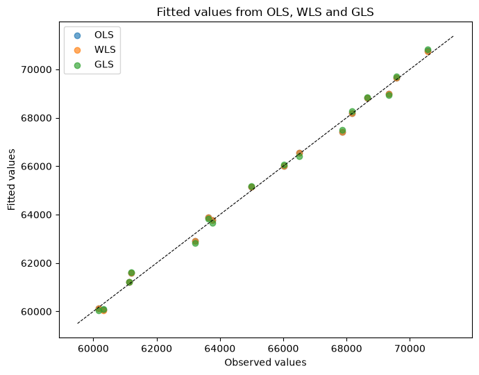
Finally, a quick visual comparison of the fitted values produced by the three estimators. We scatter the fitted values from OLS, WLS and GLS against the observed values on a single plot, using a distinct color for each estimator. The closer the points hug the dashed identity line, the better the fit.
[8]:
colors = ["#1f77b4", "#ff7f0e", "#2ca02c"]
fig, ax = plt.subplots(figsize=(7, 5.5))
for name, res, color in zip(names, results, colors, strict=False):
    ax.scatter(data.endog, res.fittedvalues, alpha=0.65, label=name, color=color)
ymin, ymax = ax.get_ylim()
ax.plot([ymin, ymax], [ymin, ymax], color="k", linestyle="--", linewidth=0.8)
ax.set_xlabel("Observed values")
ax.set_ylabel("Fitted values")
ax.set_title("Fitted values from OLS, WLS and GLS")
ax.legend()
plt.tight_layout()
plt.show()
Summary#
In this example the GLS estimator, which accounts for the serial correlation in the residuals, has the lowest AIC and BIC of the three models, also after counting the estimated \(\rho\), but the differences are small. The R-squared of the original observations is almost the same for the three models, and OLS has the largest by construction. The nested-model tests show that ARMED is a statistically significant predictor, so it should be kept in the model.
The key takeaway: for nested models compare_lr_test and compare_f_test give you a formal answer, and for other models the information criteria (AIC/BIC) can be used if the likelihoods are for the same data and all estimated parameters are counted.