ARIMA with Seasonal Differencing Using Alternative Estimators

The ARIMA class supports several parameter estimation methods beyond the default statespace approach: hannan_rissanen, yule_walker, burg, and innovations. These methods are faster and do not require numerical optimisation, making them useful for quick estimation or as starting-value generators.

Previously, all four methods rejected any model with a non-zero seasonal period — even models whose only seasonal component is differencing (i.e. seasonal_order=(0, D, 0, s) with D > 0). This notebook demonstrates that they now correctly handle seasonal differencing while still raising a clear error for seasonal AR or MA terms.

%matplotlib inline

import warnings

import matplotlib.pyplot as plt
import pandas as pd
import statsmodels.api as sm
from statsmodels.tsa.arima.model import ARIMA

plt.rc("figure", figsize=(14, 5))
plt.rc("font", size=12)
warnings.filterwarnings("ignore")

Data: Mauna Loa Atmospheric CO₂

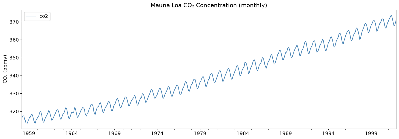
We use the classic Keeling Curve dataset, which records monthly mean atmospheric CO₂ concentrations (in parts per million by volume) measured at the Mauna Loa Observatory, Hawaii. The series exhibits two clear features:

• A long-run upward trend driven by fossil-fuel emissions.

• A strong annual seasonal cycle caused by Northern Hemisphere plant growth (CO₂ is drawn down each summer and rises each winter).

These features make the CO₂ series a natural candidate for a model with both regular and seasonal differencing.

co2 = sm.datasets.co2.load_pandas().data
co2 = co2.resample("ME").mean().ffill()   # resample to month-end, fill one gap
print(sm.datasets.co2.NOTE)

::

    Number of observations: 2225
    Number of variables: 2
    Variable name definitions:

        date - sample date in YYMMDD format
        co2 - CO2 Concentration ppmv

    The data returned by load_pandas contains the dates as the index.

fig, ax = plt.subplots()
co2.plot(ax=ax, color="steelblue")
ax.set_title("Mauna Loa CO₂ Concentration (monthly)")
ax.set_ylabel("CO₂ (ppmv)")
ax.set_xlabel("")
plt.tight_layout()

Choosing a Model

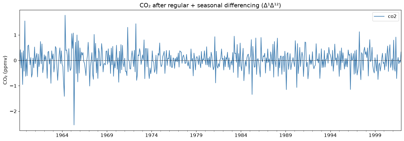
A single seasonal difference (D=1, s=12) removes the annual seasonal pattern, and a single regular difference (d=1) removes the linear trend. After both differences the series is approximately stationary, so low-order AR and MA terms are sufficient.

We use ARIMA(1, 1, 1)(0, 1, 0, 12) as the main specification. For estimators that only support pure-AR models (yule_walker, burg) we use ARIMA(2, 0, 0)(0, 1, 0, 12) instead.

co2_diff = co2.diff().diff(12).dropna()

fig, ax = plt.subplots()
co2_diff.plot(ax=ax, color="steelblue")
ax.set_title("CO₂ after regular + seasonal differencing (Δ¹Δ¹²)")
ax.set_ylabel("CO₂ (ppmv)")
ax.set_xlabel("")
ax.axhline(0, color="black", linewidth=0.8, linestyle="--")
plt.tight_layout()

Fitting with Alternative Estimators

Hannan-Rissanen

hannan_rissanen fits ARMA models via a three-step least-squares procedure. It is fast and closed-form. We pass seasonal_order=(0, 1, 0, 12) so the series is seasonally differenced before estimation.

res_hr = ARIMA(co2, order=(1, 1, 1), seasonal_order=(0, 1, 0, 12)).fit(
    method="hannan_rissanen"
)
print(res_hr.params.round(4))

ar.L1     0.1481
ma.L1    -0.4870
sigma2    0.1796
dtype: float64

Yule-Walker

yule_walker is limited to pure-AR models but supports seasonal differencing in the same way.

res_yw = ARIMA(co2, order=(2, 0, 0), seasonal_order=(0, 1, 0, 12)).fit(
    method="yule_walker"
)
print(res_yw.params.round(4))

ar.L1     0.6965
ar.L2     0.2691
sigma2    0.1831
dtype: float64

Statespace (reference)

We also fit the same ARIMA(1,1,1)(0,1,0,12) specification with the default statespace method. This produces full MLE estimates with standard errors, serving as a numerical reference for the alternative estimators.

res_ss = ARIMA(co2, order=(1, 1, 1), seasonal_order=(0, 1, 0, 12)).fit(
    method="statespace"
)
res_ss.summary()

SARIMAX Results

Dep. Variable:	co2	No. Observations:	526
Model:	ARIMA(1, 1, 1)x(0, 1, [], 12)	Log Likelihood	-279.436
Date:	Wed, 15 Jul 2026	AIC	564.871
Time:	16:59:12	BIC	577.592
Sample:	03-31-1958	HQIC	569.857
	- 12-31-2001
Covariance Type:	opg

	coef	std err	z	P>|z|	[0.025	0.975]
ar.L1	0.2684	0.101	2.648	0.008	0.070	0.467
ma.L1	-0.6171	0.086	-7.202	0.000	-0.785	-0.449
sigma2	0.1740	0.009	20.213	0.000	0.157	0.191

Ljung-Box (L1) (Q):	0.02	Jarque-Bera (JB):	44.79
Prob(Q):	0.89	Prob(JB):	0.00
Heteroskedasticity (H):	0.58	Skew:	-0.15
Prob(H) (two-sided):	0.00	Kurtosis:	4.41

Warnings:
[1] Covariance matrix calculated using the outer product of gradients (complex-step).

Comparing Parameter Estimates

The alternative estimators are consistent but not efficient — they trade some accuracy for speed. The table below compares the AR and MA coefficients from Hannan-Rissanen against the statespace MLE reference.

comparison = pd.DataFrame({
    "hannan_rissanen": res_hr.params.drop("sigma2").round(4),
    "statespace (MLE)": res_ss.params.drop("sigma2").round(4),
})
print(comparison.to_string())

       hannan_rissanen  statespace (MLE)
ar.L1           0.1481            0.2684
ma.L1          -0.4870           -0.6171

Residual Diagnostics

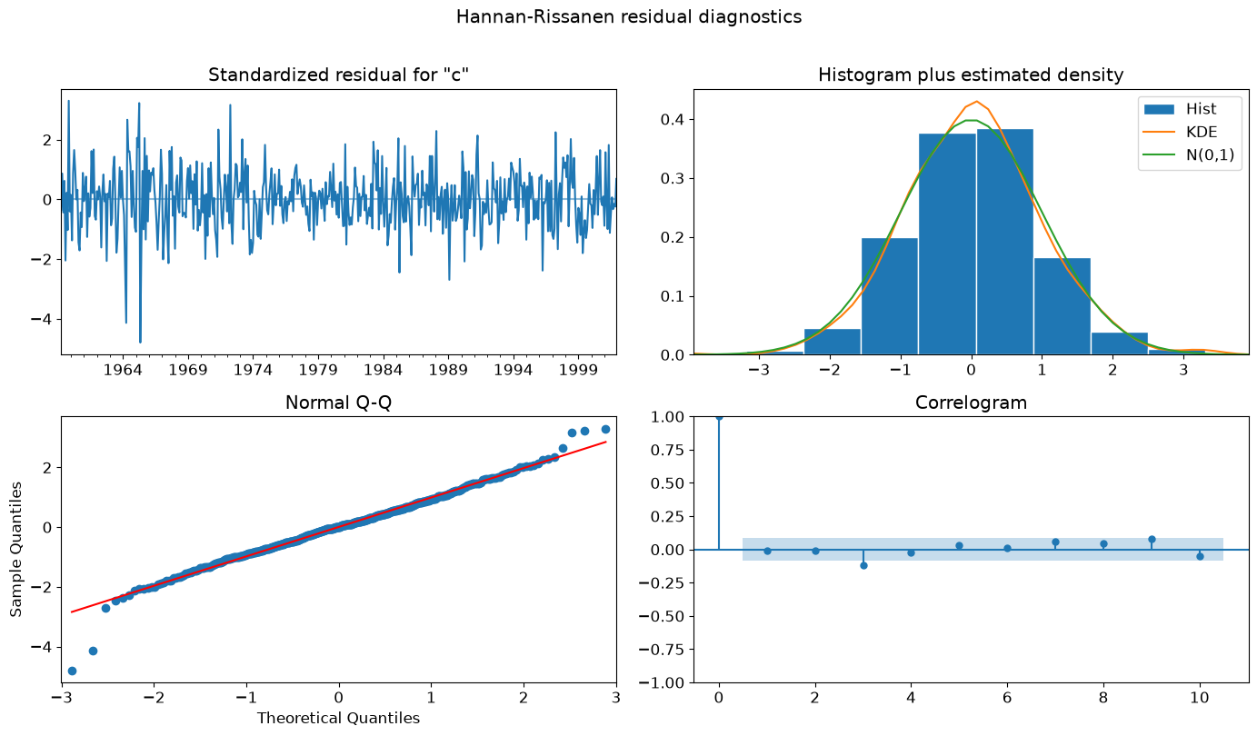
A quick look at the Hannan-Rissanen residuals confirms there is no remaining structure in the series.

fig = res_hr.plot_diagnostics(figsize=(14, 8))
fig.suptitle("Hannan-Rissanen residual diagnostics", y=1.01)
plt.tight_layout()

What Is Still Not Supported

Seasonal AR and MA terms (P > 0 or Q > 0) require the full statespace machinery. The alternative estimators will raise a ValueError with a clear message:

try:
    ARIMA(co2, order=(1, 0, 0), seasonal_order=(1, 0, 0, 12)).fit(
        method="hannan_rissanen"
    )
except ValueError as e:
    print(type(e).__name__, ":", e)

ValueError : Hannan-Rissanen estimator does not support seasonal AR or MA components.

Summary

Estimator	Seasonal diff (D>0)	Seasonal AR/MA (P,Q>0)
hannan_rissanen	✓ supported	✗ raises ValueError
yule_walker	✓ supported	✗ raises ValueError
burg	✓ supported	✗ raises ValueError
innovations	✓ supported	✗ raises ValueError
innovations_mle	✓ supported	✓ supported
statespace	✓ supported	✓ supported

For full SARIMA models with seasonal AR or MA components, use method="statespace" or method="innovations_mle".